


目录
Classification and Representation
Simplified Cost Function and Gradient Descent
Solving the Problem of Overfitting
Regularized Logistic Regression
第三周
Classification and Representation
Classification
分类问题很多是判断物体属不属于某个标签,比如收到的是否是垃圾邮件。介绍一个Sigmoid 函数 or 逻辑函数,定义如下:
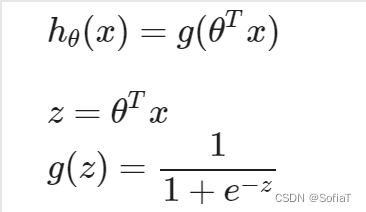
可以用这个函数在给定x和θ的情况下,表示y为1的概率为多少,图像类似下图:
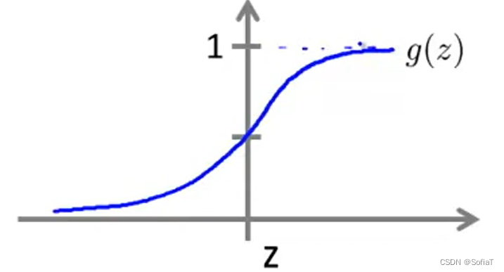
可以看到,sigmoid函数的范围在(0,1)。不采用一元方程之类的模型,其值域远远超出问题所需,导致误差过大。
Logistic Regression Model
Cost Function
为了保证J(θ)求偏导得出的函数是convex的、适合梯度下降法,这里采用下图方式来做Cost计算:
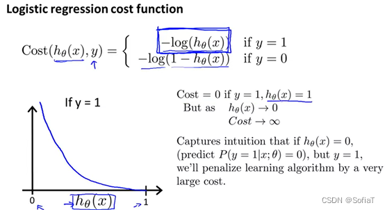
如图当y=1时,如果预测值接近0(表示y为1的概率接近0),那么误差将接近于无限大;如果预测值接近1,那么误差将接近于0。采用该方法有两种好处:
1. 能正确地判断当前值距离预测值的误差
2. 能把梯度下降函数平滑
Simplified Cost Function and Gradient Descent
通过公式,具体求导细节可参考博客中的2.对损失函数求导并得出迭代公式
部分,得到化简后的结果如下:
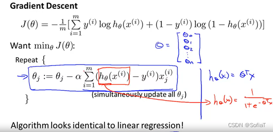
虽然形式之前学过的线性回归θ表达式,但是注意到这里的hθ(xi)的定义,明显与线性回归内的多项式不同,需要计算sigmoid函数。
其向量化表示如下:
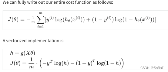

这里一开始我没搞懂h=g(Xθ)到J(θ)的简化转化,最初我理解g(Xθ)是,但是看了扩展阅读:e的矩阵指数,发现如果这样理解,既不符合e的矩阵指数定义(要求是方阵),也不符合后续计算的数据格式要求和实际定义。这里的g(Xθ)实际指的是下面这种简写替换,实际是一个向量:
并不真的是指代e的矩阵指数。
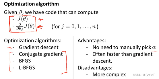
Advanced Optimization
Coursera | Online Courses & Credentials From Top Educators. Join for Free | Coursera
通过利用fminunc等函数可以简化梯度下降的过程,只需要实现cost function和J(θ)对θ的偏导即可。如:
options = optimset('GradObj', 'on', 'MaxIter', 200);
[theta, J, exit_flag] = ...
fminunc(@(t)(lrCostFunction(t, X, y, lambda)), theta, options);
Multiclass Classification
One-vs-all
如标题所示,如果遇到了标签不是简单的非1即0情况,y有三种、四种乃至n种离散的可能结果,那就把它们分为n个logistic回归
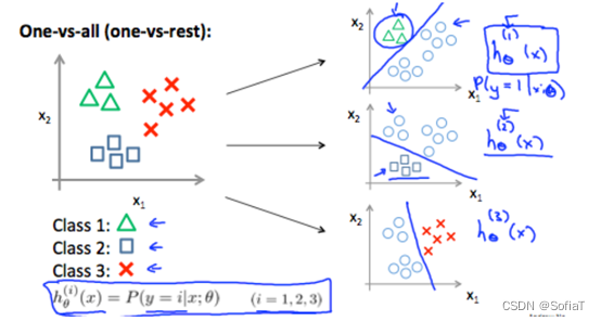
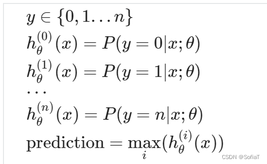
最终预测值为所有可能性中最大的那个。
Solving the Problem of Overfitting
The Problem of Overfitting
正如在线性拟合中会出现过拟合一样,逻辑回归中也存在过拟合现象,其原理是一致的。下图为逻辑回归中的一些欠拟合、正常拟合、过拟合例子:
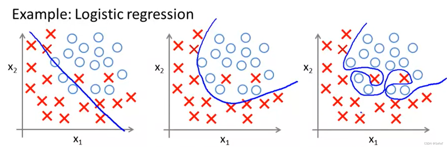
欠拟合 Underfitting, or high bias:模型过于简单,或采用的特征过少,不能很好的预测训练集和测试集。
过拟合 Overfitting, or high variance:模型过于复杂,或采用了大量无关的特征,能很好的预测训练集,但是在测试集上表现得更差
对于过拟合,可以按照以下方式进行改进:
1. 减少特征值数量:可以手动剔除无关特征,或者使用一种算法(之后会见到)
2. 正则化:使θ曲线的变化更加平滑
ps:在李宏毅老师的课里也提到了过拟合,注意过拟合前提是对训练集匹配的很好,不要只看训练集的效果就判断是过拟合。
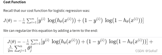
Cost Function
它实现的效果是使曲线更加平滑。通过更改Cost Function如下式:
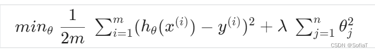
可以看到把θ添加到Cost Function之后,要想减少误差,就需要更小的θ值, 更小的θ值让曲线变化的更平滑、更不剧烈。达到的效果如下图(蓝色为CostFunc添加θ前的预测函数、紫色为添加后):

Regularized Linear Regression
与之前线性回归中的内容基本一致,新增关于Normal Function的技巧:
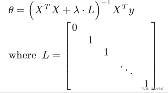
可以使直接计算出来的θx曲线更加平滑。
Regularized Logistic Regression
与线性回归中做的操作类似。
ex-2
主函数代码注释:
%% Machine Learning Online Class - Exercise 2: Logistic Regression
%  简介
%  ------------
%     需要完成的函数为:
%     sigmoid.m
%     costFunction.m
%     predict.m
%     costFunctionReg.m

% 初始化:删除当前环境下的临时变量、关闭之前的绘图窗口、清除当前命令行log
clear ; close all; clc

% 加载训练数据'ex2data1.txt',有三列,前两列为特征,第三列为标签
data = load('ex2data1.txt');
X = data(:, [1, 2]); y = data(:, 3);

%% ==================== Part 1: 绘图 ====================
%  观察现有数据集特征,以便找到合适的模型

% 用+表示标签为真的点,-表示标签为假的点(这里刚好只有两个feature,所以可以画个二维平面图)
fprintf(['Plotting data with + indicating (y = 1) examples and o ' ...
         'indicating (y = 0) examples.\n']);
% 需用到finx、plot函数来完成
plotData(X, y);

hold on;
% 横纵坐标表示的意义
xlabel('Exam 1 score')
ylabel('Exam 2 score')

% 图例,右上角的注释
legend('Admitted', 'Not admitted')
hold off;

fprintf('\nProgram paused. Press enter to continue.\n');
pause;


%% ============ Part 2: 计算 Cost 和 Gradient ============
[m, n] = size(X);

% 新增一列全为1的x0,用来对应θ0
X = [ones(m, 1) X];

% 初始θ为一列全为1的向量
initial_theta = zeros(n + 1, 1);

% costFunction计算J为cost,grad为梯度下降方向
[cost, grad] = costFunction(initial_theta, X, y);

% 一些用来辅助判断函数是否正确的log
fprintf('Cost at initial theta (zeros): %f\n', cost);
fprintf('Expected cost (approx): 0.693\n');
fprintf('Gradient at initial theta (zeros): \n');
fprintf(' %f \n', grad);
fprintf('Expected gradients (approx):\n -0.1000\n -12.0092\n -11.2628\n');

% 一个用来辅助判断costFunction是否正确的θ
test_theta = [-24; 0.2; 0.2];
[cost, grad] = costFunction(test_theta, X, y);

fprintf('\nCost at test theta: %f\n', cost);
fprintf('Expected cost (approx): 0.218\n');
fprintf('Gradient at test theta: \n');
fprintf(' %f \n', grad);
fprintf('Expected gradients (approx):\n 0.043\n 2.566\n 2.647\n');

fprintf('\nProgram paused. Press enter to continue.\n');
pause;


%% ============= Part 3: 通过fminunc优化处理  =============
%  使用octave内置函数 (fminunc) 简化梯度下降步骤

% fminunc的设置(详见 help optimset)
%% GradObj:默认为off,当on时,要被迭代至值最小化的函数一定会返回两个return值,其中第二个return是该X点的梯度或者一阶导数
%% MaxIter:optimization停止前最多迭代多少次
options = optimset('GradObj', 'on', 'MaxIter', 400);

% [X, FVAL, INFO, OUTPUT, GRAD, HESS] = fminunc (FCN, X0, OPTIONS)
% On return, X 是当FCN(X)最小时的X and FVAL是VCN(X)的值
[theta, cost] = ...
	fminunc(@(t)(costFunction(t, X, y)), initial_theta, options);

% 一些用来辅助判断函数是否正确的log
fprintf('Cost at theta found by fminunc: %f\n', cost);
fprintf('Expected cost (approx): 0.203\n');
fprintf('theta: \n');
fprintf(' %f \n', theta);
fprintf('Expected theta (approx):\n');
fprintf(' -25.161\n 0.206\n 0.201\n');

% Plot Boundary
plotDecisionBoundary(theta, X, y);

% Put some labels
hold on;
xlabel('Exam 1 score')
ylabel('Exam 2 score')
legend('Admitted', 'Not admitted')
hold off;

fprintf('\nProgram paused. Press enter to continue.\n');
pause;

%% ============== Part 4: Predict and Accuracies ==============
%  一个单例数据试试θ能预测出的概率是多少

prob = sigmoid([1 45 85] * theta);
fprintf(['For a student with scores 45 and 85, we predict an admission ' ...
         'probability of %f\n'], prob);
fprintf('Expected value: 0.775 +/- 0.002\n\n');

% 计算预测后的概率值,如果大于等于0.5则认为是真,反之认为是假
p = predict(theta, X);

fprintf('Train Accuracy: %f\n', mean(double(p == y)) * 100);
fprintf('Expected accuracy (approx): 89.0\n');
fprintf('\n');
plotDecisionBoundary函数注释:
function plotDecisionBoundary(theta, X, y)
%PLOTDECISIONBOUNDARY Plots the data points X and y into a new figure with
%the decision boundary defined by theta
%   PLOTDECISIONBOUNDARY(theta, X,y) plots the data points with + for the
%   positive examples and o for the negative examples. X is assumed to be
%   a either
%   1) Mx3 matrix, where the first column is an all-ones column for the
%      intercept.
%   2) MxN, N>3 matrix, where the first column is all-ones

% Plot Data
plotData(X(:,2:3), y);
hold on

% 这里把画图分为ex2和ex2_reg这两种情况来考虑
% ex2的feature大小为Mx3,是二维平面情形,所以只用画一条直线即可
if size(X, 2) <= 3
    % min(X(:,2))是X中第二列元素的最小值,max(X(:,2))是X中第二列元素的最大值
    % 刚好比数据集的范围大一点
    plot_x = [min(X(:,2))-2,  max(X(:,2))+2];

    % 这里绘制的是x1与x2的平面图,所以plot_x是x1,、plot_y是x2
    % 根据之前预设的model,得到直线方程为:θ0+θ1*x1+θ2*x2=0 是model预测的分割线
    % 现在已知x1,利用方程求出x2即可
    plot_y = (-1./theta(3)).*(theta(2).*plot_x + theta(1));

    % Plot, and adjust axes for better viewing
    plot(plot_x, plot_y)

    % Legend, specific for the exercise
    legend('Admitted', 'Not admitted', 'Decision Boundary')
    axis([30, 100, 30, 100])
else
    % ex2的feature大小为MxN,是从2维映射到N维的
    % Here is the grid range
    u = linspace(-1, 1.5, 50);
    v = linspace(-1, 1.5, 50);

    z = zeros(length(u), length(v));
    % Evaluate z = theta*x 通过theta和map到的feature计算出每个点对应的theta
    for i = 1:length(u)
        for j = 1:length(v)
            z(i,j) = mapFeature(u(i), v(j))*theta;
        end
    end
    z = z'; % important to transpose z before calling contour

    %  -- contour (X, Y, Z, VN) 绘制等高线图的方法

    % Plot z = 0
    % 参考matlab的博客<url>https://blog.csdn.net/xuxinrk/article/details/80841879</url>,[0,0]的含义为:
    % 要在特定值位置显示单个等高线,请将 v 定义为一个二元素向量,并且两个元素都等于所需的等高线层级。
    % 当z为0时,对应h(z)为0.5,即可代表预测的分界线,这里用[0, 0]是绘制等高线的格式要求
    contour(u, v, z, [0, 0], 'LineWidth', 2)
end
hold off

end
总结一下,主要流程:
初始化、导入数据 → 绘图观察 → 新增θ和x0 → 进行梯度下降 → 观察预测数据并优化 → 得到预测正确概率
遇到的问题一:
!! Submission failed: theta(28): out of bound 3 (dimensions are 3x1)


Function: costFunctionReg
FileName: costFunctionReg.m
LineNumber: 20

Please correct your code and resubmit.
原因:在剔除θ0对梯度下降的影响时,我用了硬编码去得到theta数组的其他部分,导致submit的自动检测扫到了我数组越界。
遇到的问题二:
运行ex-2的时候命令行窗口log了一堆中间变量。
一开始以为是编辑器的默认setting被我动了,后来发现是sigmoid函数有一行赋值没加分号,所以按行执行的时候直接log出来了。
遇到的问题三:
predict模组本地测试和提供的数据一致都是83.1 (approx),submit上去0分。
仔细读了predict的注释,发现自己把预测函数的定义弄错了,预测函数是1/(1+e^(hθ(x))),我只计算成了hθ(x),但是神奇的是提供的测试数据算得数据和Expected的近似,导致我一开始没发现这个错误。
遇到问题四:
costFunctionReg函数输出和fprintf的值不一致。
为了让曲线平滑,J新增了λθ^2,偏导新增了λθ,但是其中不应该有θ0的值被计算在内,因为x0默认为1,θ0是一个特殊的常量系数。在计算中把中间变量的θ0赋值为0即可。(在后面的ex-3中提到一个更简洁的写法θ(:, 2:end))
遇到的问题四:
debug,可以看命令行里面的提示,常用的有dbclear、dbcont等。GUI上面可以加断点和直接看变量,不过命令行的debug可以自己把中间计算输出,感觉是解释型语言的一个优点。


 3951
3951


 被折叠的 条评论
为什么被折叠?
被折叠的 条评论
为什么被折叠?
 到【灌水乐园】发言


