我的实战项目——用户评分数据探索

项目简介

-此数据集为一商品网站大约16万用户在4年内对网站商品的评分数据，每条评分记录都有时间戳（隐匿了具体时间，只保证顺序不变），评分分为5级，1分最低，5分最高。

DataExploration

数据字段：uid——用户id，iid——商品id，score——用户评分，time——评分时间。
数据集包含33177269条数据，用户数157949，商品数14620。

import numpy as np
import pandas as pd
train = pd.read_csv("train.csv")
print(train.shape)
train.head()

数据量过大：尝试用迭代器读取一部分进行观察

chunks = pd.read_csv('train.csv',iterator = True)
chunk = chunks.get_chunk(100)
print(chunk)
type(chunk)

将数据集均分为十份：尝试分块进行探索，后期没用上。

dur = int(len(train)/10)
ifrom = 0
idx = 0
while ifrom < len(train):
    ito = ifrom + dur
    data = train[ifrom:ito]
    print("from ", ifrom, "to ", (ito-1))
    print(idx)
    data.to_csv('train_' + str(idx) + '.csv', index=False)
    ifrom = ito
    idx += 1

Exolore each feature

1.uid

train.uid.describe()
user_group = train.groupby('uid')

可以看出用户数共157949，编号从0到223969

def user_attr_trans(df):
    result = pd.Series(index=['item_count','item_count_per_day',
                              'score_mean','score_std',
                              'period','time_min','time_max','latest_period'])
    result['item_count'] = df.iid.count()
    result['item-count_per_day'] = df.iid.count/(df.time.max()-df.time.min()+1)
    result['score_mean'] = df.score.mean()
    result['score_std'] = df.score.std()
    result['time_max'] = df.time.max()
    result['time_min'] = df.time.min()
    result['period'] = df.time.max()-df.time.min()+1
    result['latest_period'] = 1347 - df.time.max()
    return result

user_info = user_group.apply(user_attr_trans)
user_info.to_csv('user_train')
user_info = pd.read_csv("user_train.csv")

考虑直接用函数将数据从不同维度计算，生成新的数据集，电脑内存带不动，所以以下是我单个分析结果。

1.1 商品维度

1.1.1 单个用户评论总数

item_count = user_group.iid.count()
item_count.describe()
plt.scatter(item_count.index,item_count.values)

print('总评论数大于500的人数%d'%item_count[item_count>500].shape[0])
print('总评论数大于500的人数占比{:.3f}'.format(item_count[item_count>500].shape[0]/item_count.shape[0]))

总评论数大于500的人数16966
总评论数大于500的人数占比0.107

1.1.2 每个用户每天评论数

#每个用户每天评论数--日活跃度
item_count_per_day = item_count/period
item_count_per_day.describe()  #平均值为1.5，最大值为800，明显存在异常值
plt.scatter(item_count_per_day.index,item_count_per_day.values)

print('每日评论数大于100的人数%d'%item_count_per_day[item_count_per_day>100].shape[0])#可能为异常值

共有209人每日评论超过100条，与总样本数相差较大，可忽略不计

##每个用户每周评论数--周活跃度
item_count_per_week = item_count/week
item_count_per_week.describe()

#每个用户每月评论数--月活跃度
item_count_per_month = item_count/month
item_count_per_month.describe()

1.2 时间维度

1.2.1 第一次评论时间

#第一次评论时间---注册时间——新增用户
frist_time = user_group.time.min()
frist_time.describe()
frist_time.hist(bins=100)

可以明显看出用户的增长，且增长幅度随时间的推移逐渐增大，说明平台运营良好。

1.2.2 最后一次评论时间

#最后一次评论时间--离开时间
last_time = user_group.time.max()
last_time.describe()
last_time.hist(bins=100)

#最后一次评论截止到取数时间有多少天了——结合商品购买周期可进行流失判断
latest_time = 1347 -last_time
latest_time.describe()

print('末次评论时间超过30天的人数%d'%latest_time[latest_time>30].shape[0])
print('末次评论时间超过30天的人数占比{:.3f}'.format(latest_time [latest_time>30].shape[0]/latest_time.shape[0]))

末次评论时间超过30天的人数仅占0.12，初步判断留存较高

1.2.3 用户活跃天数

#用户活跃天数
period = user_group.time.max()-user_group.time.min()+1
period.describe()
period.hist(bins=150)

print('活跃天数超过1000的人数%d'%period [period >1000].shape[0])
print('活跃天数超过1000的人数占比{:.3f}'.format(period[period>1000].shape[0]/period.shape[0]))

网站的忠实用户，需要重点维护

#用户活跃周数
week = (user_group.time.max()-user_group.time.min()+1)/7
week.describe()

#用户活跃月数
month = (user_group.time.max()-user_group.time.min()+1)/30
month.describe()

1.3 评分维度

1.3.1 每个用户打分平均分

#每个用户打分平均分
score_mean = user_group.score.mean()
score_mean.hist(bins=150)#评分接近正态分布

print('平均分大于3的人数%d'%score_mean [score_mean >3].shape[0])
print('平均分大于3的人数占比{:.3f}'.format(score_mean[score_mean>3].shape[0]/score_mean.shape[0]))

平均分大于3的人数144552
平均分大于3的人数占比0.915
百分之90的人对商品较为满意，说明网站用户满意度高

print('平均分大于4的人数%d'%score_mean [score_mean >4].shape[0])
print('平均分大于4的人数占比{:.3f}'.format(score_mean[score_mean>4].shape[0]/score_mean.shape[0]))

平均分大于4的人数23004
平均分大于4的人数占比0.146
百分之14的人对商品非常满意

1.3.2 每个用户打分标准差

#每个用户打分标准差——看异常
score_std = user_group.score.std()
score_std.describe()

score_std[score_std==0].count()#135个人对所有商品评分不变，可能为异常值

数据合并

data = {'item_count':item_count,'item_count_per_day':item_count_per_day,'score_mean':score_mean,'score_std':score_std,
       'period':period,'frist_time':frist_time,'last_time':last_time,'latest_time':latest_time}
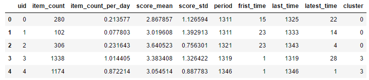
user_info = pd.DataFrame(data,index=item_count.index)
user_info.head()

user_info.to_csv('user_info')

用户聚类

user_info = pd.read_csv('user_info')
user_cluster = user_info[['item_count','score_mean','period']]
user_cluster.head()

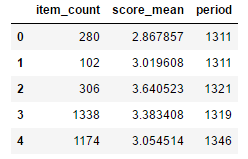
因为数据维度较少，所以优先使用所有维度进行聚类，但是实际情况还需要根据业务解释需求进行聚类指标和类数的划分。目前选择的商品评论总数，评分均值，活跃天数，是我认为更易于解释的变量。

#标准化
from sklearn.preprocessing import StandardScaler
scaler = StandardScaler()
user_cluster_std = scaler.fit_transform(user_cluster)
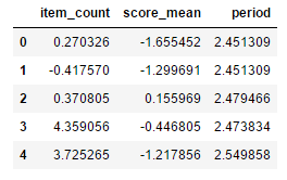
user_cluster_std = pd.DataFrame(user_cluster_std,
                               columns=['item_count','score_mean','period'])
user_cluster_std.head()

# Calinski-Harabasz法找出效果最好的簇数 ——无标签情况下
from sklearn.cluster import KMeans
from sklearn.metrics import calinski_harabaz_score
for i in range(2,8):
    kmeans=KMeans(n_clusters=i,random_state=123).fit(user_cluster_std)
    score=calinski_harabaz_score(user_cluster_std,kmeans.labels_)
    print('用户数据聚%d类calinski_harabaz指数为：%f'%(i,score))

用户数据聚2类calinski_harabaz指数为：71063.925300
用户数据聚3类calinski_harabaz指数为：67463.643219
用户数据聚4类calinski_harabaz指数为：78146.284415
用户数据聚5类calinski_harabaz指数为：71558.629962
用户数据聚6类calinski_harabaz指数为：68510.829695
用户数据聚7类calinski_harabaz指数为：67311.114270
calinski_harabaz_score分数越高效果越好，因此从数据中可以得出用户聚4类效果最好。

from sklearn.cluster import KMeans
kmeans=KMeans(n_clusters=4,random_state=123).fit(user_cluster_std)
#centers = kmeans.cluster_centers_
predictions = kmeans.predict(user_cluster_std)
user_info['cluster']=predictions
user_info.head()

#每类人群分布
user_1 = user_info[user_info.cluster==0].shape[0]/user_info.cluster.count()
user_2 = user_info[user_info.cluster==1].shape[0]/user_info.cluster.count()
user_3 = user_info[user_info.cluster==2].shape[0]/user_info.cluster.count()
user_4 = user_info[user_info.cluster==3].shape[0]/user_info.cluster.count()
print(user_1,user_2,user_3,user_4,)

# 饼图
labels = '第一类用户','第二类用户','第三类用户','第四类用户'
sizes = [user_1*100, user_2*100, user_3*100,user_4*100]
explode = (0,0,0,0)
plt.pie(sizes,autopct='%0.1f%%', labels=labels,explode=explode,shadow=False)
plt.title('用户聚类')
plt.show()

分群探索

user_1 = user_info[user_info.cluster==0]
user_2 = user_info[user_info.cluster==1]
user_3 = user_info[user_info.cluster==2]
user_4 = user_info[user_info.cluster==3]

商品评论总数

fig,axes = plt.subplots(1,4,figsize=(16,4))
user_1.item_count.plot(ax=axes[0],kind='box',title='1')
user_2.item_count.plot(ax=axes[1],kind='box',title='2')
user_3.item_count.plot(ax=axes[2],kind='box',title='3')
user_4.item_count.plot(ax=axes[3],kind='box',title='4')

购买数量——粗略认为购买数量越多，价值越高
第四类购买数量最多，因此应该归为贵宾用户

商品评分均值

fig,axes = plt.subplots(1,4,figsize=(16,4))
user_1.score_mean.plot(ax=axes[0],kind='box',title='1')
user_2.score_mean.plot(ax=axes[1],kind='box',title='2')
user_3.score_mean.plot(ax=axes[2],kind='box',title='3')
user_4.score_mean.plot(ax=axes[3],kind='box',title='4')

评分均值——粗略认为评分均值代表用户满意度
第三类人群评分最高，对网站最为满意

用户活跃天数

fig,axes = plt.subplots(1,4,figsize=(16,4))
user_1.period.plot(ax=axes[0],kind='box',title='1')
user_2.period.plot(ax=axes[1],kind='box',title='2')
user_3.period.plot(ax=axes[2],kind='box',title='3')
user_4.period.plot(ax=axes[3],kind='box',title='4')

留存时间——粗略认为活跃天数代表用户留存时间，代表忠诚度
第二类人群时间最长，对网站忠诚度最高。
PS：具体的用户分群解释，应该在相应业务场景中实现。

2.iid

train.iid.describe()
item_group = train.groupby('iid')

2.1 用户维度

2.1.1 单个商品评论总数

#评分人数
user_count = item_group.uid.count()
user_count.describe()
plt.scatter(user_count.index,user_count.values)

#热门商品，平均每天都有人评价
print('评分数大于1347的商品%d'%user_count [user_count>1347].shape[0])
print('评分数大于1347的商品占比{:.3f}'.format(user_count[user_count>1347].shape[0]/user_count.shape[0]))

评分数大于1347的商品3569
评分数大于1347的商品占比0.244

#冷门商品，四年间只有小于一百个人有评价
print('评分数小于100的商品%d'%user_count [user_count<100].shape[0])
print('评分数小于100的商品占比{:.3f}'.format(user_count[user_count<100].shape[0]/user_count.shape[0]))

2.1.2 单个商品评均每日评论总数

#每日用户评分数
user_per_day = user_count/item_day
user_per_day.describe()
plt.scatter(user_per_day.index,user_per_day.values)

#热门商品，平均每天评论数大于10
print('平均每天评论数大于10的商品%d'%user_per_day[user_per_day>5].shape[0])
print('平均每天评论数大于10的商品占比{:.3f}'.format(user_per_day[user_per_day>5].shape[0]/user_per_day.shape[0]))

#每周用户评分数
user_per_week = user_count/item_week
user_per_week.describe()

2.2 时间维度

2.2.1 单个商品评论周期

#商品评分日期——天
item_day = item_group.time.max()-item_group.time.min()+1
#商品评分日期——周
item_week = (item_group.time.max()-item_group.time.min()+1)/7
#商品评分日期——月
item_month = (item_group.time.max()-item_group.time.min()+1)/30

item_day.describe()
item_day[item_day==1].count()只在一天被评价过的商品

119个商品只在一天被评价过

2.2.2 商品上新

#商品上新时间
item_new = item_group.time.min()
item_new.hist(bins=100)

item_new[item_new<100].count()

前100天有大约5000个商品上线

2.2.3 商品上线时长

#商品上线时长
exist_time = 1347-item_group.time.min()
exist_time.describe()

exist_time[exist_time==1].count()#截止时间窗口才上线的商品

exist_time.hist(bins=100)

2.2.4 商品末次评论时间间隔

#商品末次评论时间间隔
item_last = 1347 - item_group.time.max()
item_last.describe()

item_last[item_last>200].count()

最后一次评价离时间窗口200以上的商品数为183

item_last.hist(bins=10)

print('截止时间窗口30天内仍有评价的商品%d'%item_last[item_last<30].shape[0])
print('截止时间窗口30天内仍有评价的商品占比{:.3f}'.format(item_last[item_last<30].shape[0]/item_last.shape[0]))

截止时间窗口30天内仍有评价的商品13977
截止时间窗口30天内仍有评价的商品占比0.956

2.3 评分维度

2.3.1 单个商品评分均值

#商品评价均分
item_score_mean = item_group.score.mean()
item_score_mean.hist(bins=150)

item_1 = item_score_mean[item_score_mean<1].count()/14620
item_2 = item_score_mean[(item_score_mean>1)&(item_score_mean<2)].count()/14620
item_3 = item_score_mean[(item_score_mean>2)&(item_score_mean<3)].count()/14620
item_4 = item_score_mean[(item_score_mean>3)&(item_score_mean<4)].count()/14620
item_5 = item_score_mean[item_score_mean>4].count()/14620

# 饼图
labels = '一星产品','二星产品','三星产品','四星产品','五星产品'
sizes = [item_1*100, item_2*100, item_3*100,item_4*100,item_5*100]
explode = (0,0,0,0,0.1)
plt.pie(sizes,autopct='%0.1f%%', labels=labels,explode=explode,shadow=False)
plt.title('产品分级')
plt.show()

item_score_mean[item_score_mean==5].count()
item_score_mean[item_score_mean==1].count()

均值为五分的商品有46个，均值为一分的产品为7个
总体来看商品评分集中在3分到4分，商品评价较高。

2.3.2 单个商品评分方差

#商品评分标准差
item_score_std = item_group.score.std()
item_score_std.hist(bins=100)

item_score_std[item_score_std ==0].count()

30个商品评分稳定不变，整体方差在1附近，正常

数据合并

item_data = dict(user_count=user_count,user_per_day=user_per_day,exist_time=exist_time,item_last=item_last,item_score_mean=item_score_mean,item_score_std=item_score_std)
item_info = pd.DataFrame(item_data,index=user_count.index)
item_info.head()

item_info.to_csv('item_info')

商品聚类

item_info = pd.read_csv('item_info')
item_cluster = item_info[['user_count','exist_time']]
item_cluster.head()

聚类标准首先尝试的是三个维度，效果不好。后做两个维度，仅供参考。

#标准化
from sklearn.preprocessing import StandardScaler
scaler = StandardScaler()
item_cluster_std = scaler.fit_transform(item_cluster)
item_cluster_std = pd.DataFrame(item_cluster_std,
                               columns=['user_count','exist_time''item_score_mean'])
item_cluster_std.shape

# 轮廓系数评估法——易于理解，但是不适用于大数据量，因为要计算样本点与同簇的所有点以及最近的簇中所有点的平均距离
from sklearn.metrics import silhouette_score
import matplotlib.pyplot as plt
silhouettteScore = []
for i in range(2,8):
    ##构建并训练模型
    kmeans = KMeans(n_clusters = i,random_state=123).fit(item_cluster_std)
    score = silhouette_score(item_cluster_std,kmeans.labels_)
    silhouettteScore.append(score)
    print(i,score)
plt.figure(figsize=(10,6))
plt.plot(range(2,8),silhouettteScore,linewidth=1.5, linestyle="-")
plt.show()

轮廓系数不适用于如此大的数据集，因此还是使用calinski_harabaz_score进行k值选择。

# Calinski-Harabasz法找出效果最好的簇数 ——无标签情况下
from sklearn.cluster import KMeans
from sklearn.metrics import calinski_harabaz_score
for i in range(2,8):
    kmeans=KMeans(n_clusters=i,random_state=123).fit(item_cluster_std)
    score=calinski_harabaz_score(item_cluster_std,kmeans.labels_)
    print('商品聚%d类calinski_harabaz指数为：%f'%(i,score))

最终结果显示商品聚类效果不好,可能原因在于评价指标不够，对业务理解不够深入

3.time

train.time.describe()#一共1347天
time_group = train.groupby('time')

3.1 用户维度

3.1.1 每日用户评论数

user_time = time_group.uid.count()
user_time.describe()
user_time.plot()#评论数量随时间有明显趋势，网站使用人数越来越多

评论数量随时间有明显趋势，网站使用人数越来越多。评论人数出现激增的情况，推测与平台常规营销活动有关，后一个波峰没有出现之前的人数锐减情况，估计同期进行了其他活动。

fig,axes = plt.subplots(1,2,figsize=(16,4))
user_time[(user_time.index<800)&(user_time.index>700)].plot(ax=axes[0],title='1')
user_time[(user_time.index<1300)&(user_time.index>1100)].plot(ax=axes[1],title='2')

在2个时间点上有明显的提升,在750天附近实现10k->60k的提升，在1080天附近实现40k->110k的提升

3.2 商品维度

3.1.1 每日商品评论数

item_time = time_group.iid.count()
item_time.describe()

user_time.describe()

每天的商品数量与用户数量分布一致，说明每天每个用户仅对每个商品产生一次评价

3.3 评分维度

score_time = time_group.score.mean()
score_time.describe()
score_time.hist(bins=70)

每日评分均值集中在3.2到3.7之间，用户整体评价较高

数据合并

time_data = dict(user_time=user_time,score_time=score_time)
time_info = pd.DataFrame(time_data,index=user_time.index)
time_info.head()
time_info.to_csv('time_info.csv')

项目总结：从三个维度对数据集进行了剖析，很多地方不够深入，例如时间维度上可以下钻到周，月，年。对于聚类结果理解不够深入，需要多与业务知识相结合。数据的价值在于为实际业务问题提供价值，工具和方式只是辅助手段。