论文笔记：Conditional Coupled Generative Adversarial Networks for Zero-Shot Domain Adaptation

本文提出了一个比较有趣的 $ZSDA$（zero-shot domain adaptation） 的学习策略。

• 假如现在我们有两个 $UIT(StyleTransfer)$ 的任务，
  
• 原本我们可以构建两个 $CycleGAN$ 就可以解决上面的问题，或者把数据混合在一起，训练一个更高鲁棒性的 $CycleGAN$.
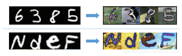
• 但实际上，有时候我们并没有右下角的目标域的图像，这时候我们希望基于上面的 $graynum.$ 和 $colornum.$ 数据集训练一个 $UIT$ 模型，它也能够应用到下面的 $grayletter\to colorletter$，但现实中，本质上仍旧是统计学的深度学习算法并不能有这样的泛化能力。
• 但如果我们知道了 $graynum.\sim grayletter$ 之间的某种对应关系 $Alig{n}_s$，那么，$colornum.\sim colorletter$ 之间也必然存在某种对应关系 $Alig{n}_t$。我们可以利用这样的对应关系来作为监督信息，代替缺失的 $colorletter$ 数据。因为存在：$$[grayletter]\to [Alig{n}_s]\to [graynum.]\to [UIT]\to [colornum.]\to [Alig{n}_t]\to [colorletter]$$

所以，理论上，这两个对应关系的限制是充分的。

---

1. CoCoGAN

首先，我们需要了解 CoGAN。

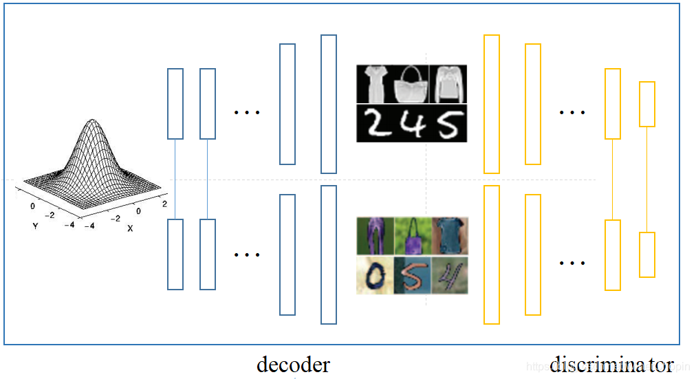
• 其基本思想是，除去样式，两个域在 content 方面是共享的，因此有两个生成器，起始于同一个 content latent space，同时两个网络共享底层（深层特征 content），异于高层（浅层特征 appearance）；同样有两个鉴别器，异于底层，共享高层。
• 因此，其目标函数为：
  $$\underset{g_1,g_2}{\max }\underset{f_1,f_2}{\min }V(f_1,f_2,g_1,g_2)\equiv {\mathbb{E}}_{x_1\sim p_{x_1}}[-\log f_1(x_1)]+{\mathbb{E}}_{z\sim p_z}[-\log (1-f_1(g_1(z)))]+{\mathbb{E}}_{x_2\sim p_{x_2}}[-\log f_2(x_2)]+{\mathbb{E}}_{z\sim p_z}[-\log (1-f_2(g_2(z)))]$$ 其中，$g_i$ 是生成器/解码器，$f_i$ 是鉴别器，$i=1,2$。

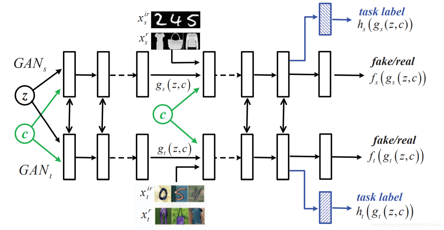
其次，我们可以理解 CoCoGAN

同样的，所谓的 $Conditional$ 是指加了一个 $c$ 用于决定让模型处理哪一个任务。

• 我们称 $graynum.\to colornum.$ 是一个（与目标任务）无关的任务（irrelevant task/$IR$）
• 我们称另一个 $grayletter\to colorletter$ 是目标/相关任务（relevant task/$R$）
• $c=0$ 时，处理 $IR$；$c=1$ 时，处理 $R$.

假如我们四个域的图像数据都有：$X_s^{ir},X_t^{ir},X_s^r,X_t^r$，那么可以直接使用 CoGAN 的对抗 loss，即，我们使用
$$\underset{g_s,g_t}{\max }\underset{f_s,f_t}{\min }V(f_s,f_t,g_s,g_t)\equiv {\mathbb{E}}_{x_s\sim p_{x_s}}[-\log f_s(x_s,c)]+{\mathbb{E}}_{z\sim p_z}[-\log (1-f_s(g_s(z,c),c))]+{\mathbb{E}}_{x_t\sim p_{x_t}}[-\log f_t(x_t,c)]+{\mathbb{E}}_{z\sim p_z}[-\log (1-f_t(g_t(z,c),c))]$$ 但实际上，第三项 $E_{x_t\sim p_{x_t}}[-\log f_t(x_t,c)]$ 只能取到 $c=0$，那么这样的训练是不充分的，结果是 $g_t$ 过分偏向于 $graynum.\to colornum.$，对于 $c=1$ 的时候，要么 $g_t(z,1)$ 也是 彩色数字，要么就什么也不是，而不是理想的彩色字母。

因此，我们需要增加新的限制——

2. Representation Alignment

在高层表征中，如 $encoder$ 和 $decoder$ 之间。

$$\underset{realdata}{\underbrace{r_s(X_s^{ir},c=0)\equiv r_t(X_t^{ir},c=0)}}\approx \underset{fakedata}{\underbrace{r_t(T(X_s^{ir}),c=0)}}$$ $$\underset{realdata}{\underbrace{r_s(X_s^r,c=1)\equiv r_t(X_t^r,c=1)}}\approx \underset{fakedata}{\underbrace{r_t(T(X_s^r),c=1)}}$$ 假如我们认为下面的对齐存在：$$r_s(X_s^{ir},c=0)\sim r_s(X_s^r,c=1)$$ 则必然会有： $$r_t(X_t^{ir},c=0)\sim r_t(X_t^r,c=1)$$ 即在两个源域 $I{R}_S$ 和 $R_S$ 以某种方式对齐，则其对应的目标域 $I{R}_T$ 和 $R_T$ 必定也以某种方式对齐。
但是由于我们没有：$r_t(X_t^r,c=1)$，所以需要近似地在合成图像 $fakedata$ 上去对齐
那如果我们现在希望用 $\mathrm{t}\mathrm{a}\mathrm{s}\mathrm{k}\mathrm{c}\mathrm{l}\mathrm{a}\mathrm{s}\mathrm{s}\mathrm{i}\mathrm{f}\mathrm{i}\mathrm{e}\mathrm{r}$ 去表达这种限制，可以有：

令 $l(.)$ 为 logistics 函数
在源域上有：$$\underset{h_s}{\max }{L}_s\equiv \underset{\mathrm{A}\mathrm{l}\mathrm{i}\mathrm{g}\mathrm{n}:realdatainS}{\underbrace{{\mathbb{E}}_{x_s\sim p_{X_s^{ir}}}[l(h_s(x_s))]+{\mathbb{E}}_{x_s\sim p_{X_s^r}}[l(h_s(x_s))]}}+\underset{\mathrm{A}\mathrm{l}\mathrm{i}\mathrm{g}\mathrm{n}:fakedatainS}{\underbrace{{\mathbb{E}}_{z\sim p_z}[l(h_s(g_s(z,c=0)))]+{\mathbb{E}}_{z\sim p_z}[l(h_s(g_s(z,c=1)))]}}$$ 同时，在目标域上有：$$\underset{h_t}{\max }{L}_t\equiv \underset{\mathrm{A}\mathrm{l}\mathrm{i}\mathrm{g}\mathrm{n}:realdatainT}{\underbrace{{\mathbb{E}}_{x_t\sim p_{X_t^{ir}}}[l(h_t(x_t))]}}+\underset{\mathrm{A}\mathrm{l}\mathrm{i}\mathrm{g}\mathrm{n}:fakedatainT}{\underbrace{{\mathbb{E}}_{z\sim p_z}[l(h_t(g_t(z,c=0)))]+{\mathbb{E}}_{z\sim p_z}[l(h_t(g_t(z,c=1)))]}}$$

---

这里有个疑问，既然在这里有 $a\times b\le \frac{a^2+b^2}{2}\le \frac{a+b}{2}$，不应该是最大化 $ab$ 则必然 最大化 $a+b$？为什么这里使用的是加法而不是乘法？
此外就是，上面的两条式子是为了好看，实际上只有 $\mathrm{A}\mathrm{l}\mathrm{i}\mathrm{g}\mathrm{n}:realdatainS$ 和 $\mathrm{A}\mathrm{l}\mathrm{i}\mathrm{g}\mathrm{n}:fakedatainT$ 是起作用的。这就是我们要对齐的东西。

这里也给出了，当我们试图对齐两个分布的时候，可以通过引入 task classifier 来拉近，目标是让两个分布的输入趋近于同一个值（在这里是 logistics 值都 $\to 1$），
但是这样会容易导致分类器对任何输入都输出是 $1$ ，这是不对的，从作者的设置来看，这个分类器的 loss 是不对的，只用在了鉴别器的优化。即：
$$(\widehat{f_s},\widehat{f_t},\widehat{h_s},\widehat{h_t})=\underset{f_s,f_t,h_s,h_t}{\mathrm{argmin}}V(f_s,f_t,\widehat{g_s},\widehat{g_t})-(L_s+L_t)$$ $$(\widehat{g_s},\widehat{g_t})=\underset{g_s,g_t}{\mathrm{argmax}}V(\widehat{f_s},\widehat{f_t},g_s,g_t)$$ 但无论如何，本文提出了一个比较好的 $DA$ 的学习策略，通过另外一组无关的任务，构建一个 $aligement$ 来作为额外的限制。

---

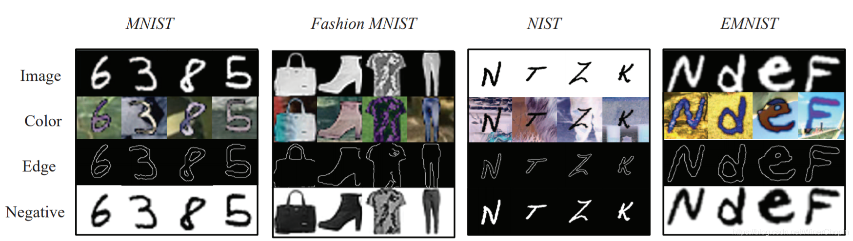
这一节我们带大家系统认识一下几个手写数据集：

总共四个数据集（ { D M , D F , D N , D E } \{ D_M,D_F,D_N,D_E \} {DM​,DF​,DN​,DE​}），但是，实际上每个数据集只有 $Gray$ 版本，我们称之为 $G-Domain$（第1行），我们需要制作不同 style 的其他 3 个 版本/domains。

• 制作 $Color$ 版本（第2行）$C-Domain$

对于每一张灰度图 $I\in {\mathbb{R}}^{h\times w\times 1}$，从彩色图像数据集 BSDS500 中选择一张图像，随机 crop 出一个块 $P\in {\mathbb{R}}^{m\times n\times 3}$，然后合并：$I_c=|I-P|$。

• 制作 $Edge$ 版本（第3行）$E-domain$

对彩色图像使用 Canny edge detector
$I_e=canny(I_c)$

• 制作 $Negative$ 版本（第4行）$N-Domain$

$I_n=255-I$

---

这一节我们介绍实验

1. baseline

• $ZDDA$ 这是另外一个唯一使用 DL 于 ZSDA 任务的方法
• $CoCoGANw/oT$ 不使用对应关系作为额外限制的 $CoCoGAN$

2. 模型评价指标

同样以最开始的例子讲述：

• 得到训练后的模型 $g_s,g_t$
• 让 $c=1$，随机采取一些随机数 $z$，获取 ${\tilde{x}}_s^r=\widehat{g_s}(z,c=1)$ 和 ${\tilde{x}}_t^r=\widehat{g_t}(z,c=1)$，我们认为 ${\tilde{x}}_s^r,{\tilde{x}}_t^r$ 是同一个字母。
• 利用已有的 $X_s^r$ 的数据集训练一个字母分类器 $C_s(x_s^r)$
• 用这个分类器 $C_s(x_s^r)$ 去对 { x ~ s r } \{\widetilde{x}_s^r\} {x sr​} 做识别，也就得到了 { x ~ t r } \{\widetilde{x}_t^r\} {x tr​} 的标签
• 用这些标签信息去训练一个字母分类器 $C_t({\tilde{x}}_t^r)$
• 用这个鉴别器去对 $X_t^r$ 作分类，根据该数据集本身的 $GT$ 计算 $C_t(x_t^r)$ 分类的准确度

3. 实验结果

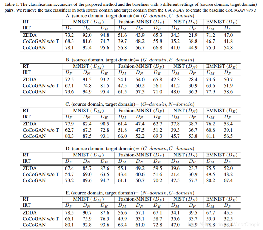
结果当然是碾压对方其他两个 $baselines$.