【Pytorch(二)】Numpy 搭建全连接神经网络

zqwlearning

已于 2022-04-14 17:45:13 修改

阅读量7.1k

点赞数 7

分类专栏： Pytorch 文章标签：神经网络 pytorch 深度学习

于 2022-01-23 19:10:45 首次发布

本文链接：https://blog.csdn.net/Ws_zqw/article/details/122655364

版权

Pytorch 专栏收录该内容

7 篇文章 11 订阅

订阅专栏

文章目录

实验一全连接神经网络FCNN
实验说明
背景知识
实验步骤

实验一全连接神经网络FCNN

实验说明

使用像 TensorFlow 和 PyTorch 这样的高级框架（deep learning framework），能够让我们方便、快速地构建各类神经网络模型。然而，理解神经网络的基本概念和内部原理对初学者来说同样重要。在本次实验中，我们将学习如何使用 Numpy 实现一个简单的全连接神经网络，并利用它来处理一个简单的分类任务，通过实践来加深对神经网络内部机制的理解。

本次实验中我们将主要使用如下两个 Python 库：

Numpy (Python 科学计算库，用于实现全连接神经网络)
Pytorch (深度学习框架，本次实验中我们将练习用它读取数据集 MNIST)

背景知识

全连接神经网络（Fully-Connected Neual Network）是一种最简单、基础的神经网络，也常叫作多层感知器（Multi-Layer Perceptron，MLP）。它的网络结构如下图所示，包含输入层 (input layer)、若干隐藏层 (hidden layers) 及输出层 (output layer)，层内神经元之间无连接，层与层之间神经元实行全连接。

在开始实验之前，请同学们回顾全连接神经网络的基本知识，包括各层的权重矩阵大小、偏置向量大小，权重、偏置、和激励之间的运算等。

实验步骤

0. 概览

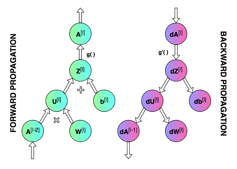
我们的目标是创建一个具有特定网络结构（层数、层大小、激活函数等）的全连接神经网络。然后训练这一神经网络并进行分类任务。实验开始前，我们先来看一下神经网络模型训练的整个过程。神经网络的训练主要包括前向传播 (forward propagation) 和反向传播 (backward propagation) ，分别如下图中所示。

前向传播过程中，我们将输入数据表示为 𝑋，网络输出表示为 𝑦_ℎ𝑎𝑡。神经网络每一层的权重矩阵用 𝑊[𝑙]表示，偏置向量用 𝑏[𝑙]表示（其中 𝑙 表示对应的层）。权重矩阵与激活向量相乘后与偏置向量相加，其结果用 𝑍[𝑙] 表示。各层最终输出的激活向量表示为 𝐴[𝑙]（𝐴[𝑙]=𝑔(𝑍[𝑙])，g为激活函数)。最后一层的输出激活向量即为神经网络输出，即𝐴[𝐿]=𝑦ℎ𝑎𝑡。最终，损失函数 (loss function) 会根据网络输出 𝑦_ℎ𝑎𝑡 与标准结果 𝑦 (golden results) 算出损失。

在反向传播过程中，我们需要用到前向传播的中间数据，包括每层的 𝐴[𝑙] 和 𝑍[𝑙]。反向传播由最后一层开始，到第一层结束。期间我们需要根据链式法则来逐层对权重 𝑊[𝑙] 和偏置 𝑏[𝑙] 计算偏导数。𝑑𝑊[𝑙] 和 𝑑𝑏[𝑙] 计算完成后，会对 𝑊[𝑙] 和 𝑏[𝑙] 进行一次更新。至此，我们就完成了一次迭代。

1. Import Numpy

import numpy as np
print(np.__version__)

1.22.1

2. 导入其他 Python 库（Import Other Libraries）

import os
from sklearn.datasets import make_moons
from sklearn.model_selection import train_test_split
import seaborn as sns
import matplotlib.pyplot as plt

3. 定义神经网络结构

我们的程序将以列表（list）的形式描述神经网络的结构（neural network architecture），之后我们可以很容易的对网络结构进行修改。列表的每一项是一个字典（dictionary），描述单个网络层的基本结构。其中，"input_dim"是该层输入信号向量的维度，"output_dim"是该层输出激活向量的维度，"activation"是该网络层所用的激活函数（如 sigmoid 和 ReLU）。

此处需要注意的是，一个网络层的输出向量同时也是下一层的输入。因此，第 m 层的"input_dim"应当与第 m-1 层"output_dim"保持一致。我们这里使用这样的表示，让大家输入两次，是为了使每一层的格式保持一致，同时让初次接触神经网络的同学们能通过亲自设置来加深对概念的理解。

稍后请同学们尝试不同的网络的结构，看看训练结果是否有什么不同，分析其趋势及原因。

例如：

增加神经网络层数
减少神经网络层数
增加或减少各层输入和输出的维度（“input_dim”, “output_dim”）
使用 Sigmoind 函数代替 ReLU

NN_ARCHITECTURE = [
    {"input_dim": 2, "output_dim": 25, "activation": "relu"},
    {"input_dim": 25, "output_dim": 50, "activation": "relu"},
    {"input_dim": 50, "output_dim": 50, "activation": "relu"},
    {"input_dim": 50, "output_dim": 25, "activation": "relu"},
    {"input_dim": 25, "output_dim": 1, "activation": "sigmoid"},
]

4. 初始化神经网络

4.1 理解权重矩阵 𝑊 和偏置向量 𝑏

定义好了网络结构，接下来就要初始化网络参数（权重及偏置）。每一层网络的权重矩阵和偏置向量如下图所示：

在这里插入图片描述

其中，𝑊 和 𝑏 分别表示权重矩阵和偏置向量。上标 [𝑙] 表示当前层的索引，下标 𝑛 表示给定层中的神经元数量。当前层 𝑊 的形状为 (𝑛[𝑙],𝑛[𝑙−1])，𝑏 的形状为 (𝑛[𝑙],1)。

请同学们注意区分上图中的矩阵、向量和标量：其中，矩阵用粗体大写字母表示，向量用粗体小写字母表示，标量用普通小写字母表示。

4.2 参数初始化方法

在理解上图的基础上，下面我们可以开始逐层初始化权重矩阵和偏置向量。神经网络参数的初始化对于模型的训练很重要，不良的参数初始值会导致梯度传播问题，降低训练速度，甚至导致模型无法收敛；而良好的参数初始值则能够加快收敛速度，并且更可能找到较优解。

下面，我们将随机赋予一个小数值给权重矩阵 𝑊 和偏置向量 𝑏 的各个元素。这里随机赋值是非常有必要的，我们不能使用完全相同的数字（例如 0）来初始化参数值，否则无法打破神经网络的对称性，会使得训练无法顺利进行。可以想见，如果所有权重都取相同值，那么不管输入是什么，隐藏层中的所有单元都会是相同的，那么反向传播算法计算出来的梯度值也是会相同的，参数更新后仍将保持一致。这种情况下，无论我们训练模型多久、网络有多深，都会陷入在初始状态中。将权重随机初始化为小数值是打破网络对称性的一个普遍方法。

那么使用较小的初值又是为什么呢？这里我们以 Sigmoid 函数作为例子来说明。请同学们观察下面 Sigmoid 函数及其导函数曲线图（蓝色-sigmoid，橙色-导数）。

可以看到，Sigmoid 导函数取值范围在(0,0.25]之间，当输入值较大时，Sigmoid 导数值趋近于0，这可能会导致权重的更新量很小，对神经网络的训练速度造成影响。所有参数使用较小的随机数是一个简单的初始化方法，它保证了我们下面将要进行的模型训练有一个足够好的起点。当然，也不是数值越小就会表现的越好。如果一个神经网络层的所有权重都非常小，那么在反向传播过程中得到的梯度值也将非常小，对于比较深的神经网络来讲，可能会导致“梯度消失”的问题。

4.3 尝试不同的参数初始化方法

同学们稍后请修改下面“init_layer”函数对应的代码，做如下尝试，看看训练结果和上面的有什么不同。

将所有参数初始化为 0

def init_layers(nn_architecture, seed = 99):
    # random seed initiation
    np.random.seed(seed)
    # number of layers in our neural network
    number_of_layers = len(nn_architecture)
    # parameters storage initiation
    params_values = {}

    # iteration over network layers
    for idx, layer in enumerate(nn_architecture):
        # note: we number network layers from 1
        layer_idx = idx + 1

        # extracting the number of units in layers
        layer_input_size = layer["input_dim"]
        layer_output_size = layer["output_dim"]

        
        # initiating the values of the W matrix and vector b for subsequent layers        

        ###############  Please finish this part  ################
        
        # [Hint]: 
        # Think about the size of W & b, and replace 'XXX' with 'layer_input_size' or 'layer_output_size' 
        # in the following code
        #    params_values['W' + str(layer_idx)] = np.random.randn(XXX, XXX) * 0.1
        #    params_values['b' + str(layer_idx)] = np.random.randn(XXX, 1) * 0.1
        
        params_values['W' + str(layer_idx)] = np.random.randn(
            layer_output_size, layer_input_size) * 0.1
        params_values['b' + str(layer_idx)] = np.random.randn(
            layer_output_size, 1) * 0.1
        
        # Have a try: if initialize W & b as 0
        # params_values['W' + str(layer_idx)] = np.zeros((layer_output_size, layer_input_size))
        # params_values['b' + str(layer_idx)] = np.zeros((layer_output_size, 1))
    
        ########################  end  ###########################

    return params_values

代码解释：由于要将权重矩阵 𝑊 和偏置向量 𝑏置为较小的随机数，因此可以使用np.random.randn()函数来完成这个工作。该函数可以生成0_{1之间的随机数向量或者矩阵，将其进行乘以0.1得到0}0.1之间的随机数。比较重要的问题是：如何确定向量或矩阵的维数。首先考虑权重矩阵 𝑊，根据所学它应该是nl x nl-1维的矩阵，其中nl是该层的神经元数量，而由“layer_output_size = layer[“output_dim”]”可知，变量layer_output_size应该是该层的输出大小，即神经元个数nl。现在寻找nl-1的值，而上一层的神经元个数等于上一层的输出，即该层的输入，该层输入大小是layer_input_size = layer[“input_dim”]。最后得出结论：nl x nl-1等价于n layer_output_size x nlayer_input_size。然后，寻找偏置向量 𝑏，根据所学它应该是nl维的向量，根据上述易知填写layer_output_size，即神经元个数。

5. 实现激活函数

激活函数虽然简单，只需一行代码就可定义，但对神经网络来说非常重要。没有激活函数的话，神经网络将变成线性函数的组合，大大降低了其表达能力。激活函数有很多种。在本次试验中，我们将选用如下两种激活函数：

Sigmoid 函数
ReLU 函数

接下来我们需要分别实现它们的正向传播（forward）和反向传播（backward）运算。Sigmoid 及 ReLU 的函数曲线和导函数曲线分别如下图中所示。请同学们阅读如下代码，并在留白处根据提示（见[Hint]）填写相应的代码，实现 ReLU 函数的正传和反传过程。

def sigmoid(Z):
    return 1/(1+np.exp(-Z))

    
def sigmoid_backward(dA, Z):
    sig = sigmoid(Z)
    return dA * sig * (1 - sig)


def relu(Z):
    
    ###############  Please finish this part  ################
    
    # [Hint]: use the following numpy function 
    #    np.maximum(XXX, XXX)
    
    return np.maximum(0,Z)

    ########################  end  ###########################


def relu_backward(dA, Z):
    
    dZ = np.array(dA, copy = True)
    
    ###############  Please finish this part  ################
    
    # [Hint]: use one-line code to mask some entries in dZ to 0
    #     dZ[XXX] = 0
    
    dZ [Z <= 0] = 0
    
    ########################  end  ###########################
    
    return dZ

代码解释：激活函数relu在正向传播时，需要将小于等于0的值映射到0，这个可以通过maximum()函数实现，将向量Z中小于等于0的值变为0。激活函数relu在反向传播时，同样需要将小于等于0的值映射到0，可以直接借助python语言的特性实现，将向量Z中小于等于0的值变为0。

6. 实现神经网络的前向传播过程

对整个神经网络来说，输入矩阵 𝑋 传入网络后将逐层向前传播，并最终在网络末端得到输出向量 𝑌_ℎ𝑎𝑡。为了让代码更易读，接下来我们将把前向传播过程拆分成两个函数来实现：

函数 6-1 (single_layer_forward_propagation)：实现单个全连接层的前向传播过程
函数 6-2 (full_forward_propagation)：基于函数 6-1，实现整个全连接神经网络的前向传播过程

6.1　函数 6-1 （single_layer_forward_propagation）：实现单个全连接层的前向传播过程

相对于反向传播来讲，神经网络层的前向传播过程是比较直观、容易理解的。这里我们假设来自上一层的输入信号为 𝐴_𝑝𝑟𝑒𝑣，当前层的权重矩阵和偏置向量分别为 𝑊_𝑐𝑢𝑟𝑟 和 𝑏_𝑐𝑢𝑟𝑟。首先，我们需要实现𝑊_𝑐𝑢𝑟𝑟和𝐴_𝑝𝑟𝑒𝑣之间的矩阵乘法运算，并将结果与𝑏_𝑐𝑢𝑟𝑟相加，得到 𝑍_𝑐𝑢𝑟𝑟。这一部分运算我们将通过 Numpy 完成。基于 NumPy，我们可以对整个网络层和整批样本一次性进行矩阵操作，无需迭代，这大大简化了我们的代码，也加速了计算。

这个运算过程如下图所示，请注意理解每个矩阵和向量的维度：

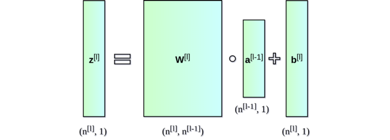
接着，我们需要对矩阵运算结果应用所选的激活函数（参数’activation’），由 𝑍_𝑐𝑢𝑟𝑟得到 𝐴_𝑐𝑢𝑟𝑟。
在这里插入图片描述

函数的输出除了经过激活函数处理的最终结果 𝐴_𝑐𝑢𝑟𝑟外，还包含中间结果 𝑍_𝑐𝑢𝑟𝑟，这是因为我们将在反向传播时用到这些中间数据。

def single_layer_forward_propagation(A_prev, W_curr, b_curr, activation="relu"):

    # calculation of the input value for the activation function

    ###############  Please finish this part  ################
    
    # [Hint]: 
    # - please implement the computation between W_curr, b_curr, and A_prev
    # - you will need to use the numpy function  ->  np.dot(XXX,XXX)
    # - the code will be like:   Z_curr = XXX
    Z_curr = np.dot(W_curr, A_prev) + b_curr

    ########################  end  ###########################

    # selection of activation function
    if activation is "relu":
        activation_func = relu
    elif activation is "sigmoid":
        activation_func = sigmoid
    else:
        raise Exception('Non-supported activation function')

    # return of calculated activation A and the intermediate Z matrix
    return activation_func(Z_curr), Z_curr

6.2　函数 6-2 (full_forward_propagation)：基于函数 6-1，实现整个神经网络的前向传播过程

在实现了单个全连接层的前向传播后，下一步就是实现整个神经网络的前向传播。神经网络的输入记为 𝑋。除了 𝑋，函数还需要网络结构的信息（nn_architecture）及初始化好的网络参数（函数 init_layers 的输出 params_values）。

需要特别注意的是，我们必须在逐层迭代时保存好反向传播需要的一些中间值，即各层的 𝐴_𝑝𝑟𝑒𝑣 和 𝑍_𝑐𝑢𝑟𝑟。这里我们将用一个 dictionary (‘memory’）来保存这些中间值。

函数的输出除了神经网络的最终输出 ‘𝐴_𝑐𝑢𝑟𝑟’ (即 𝑦_ℎ𝑎𝑡)外，还有保存有中间值的变量 ‘𝑚𝑒𝑚𝑜𝑟𝑦’。

def full_forward_propagation(X, params_values, nn_architecture):
    # creating a temporary memory to store the information needed for a backward step
    memory = {}
    # X vector is the activation for layer 0 
    A_curr = X  # shape of X: (2,900)

    # iteration over network layers
    for idx, layer in enumerate(nn_architecture):
        # we number network layers from 1
        layer_idx = idx + 1
        # transfer the activation from the previous iteration
        A_prev = A_curr

        # extraction of the activation function for the current layer
        activ_function_curr = layer["activation"]

        # extraction of W for the current layer
        W_curr = params_values["W" + str(layer_idx)]
        # extraction of b for the current layer
        b_curr = params_values["b" + str(layer_idx)]

        # calculation of activation for the current layer
        
        ###############  Please finish this part  ################
        
        # [Hint]: invoke the function single_layer_forward_propagation
        A_curr, Z_curr = single_layer_forward_propagation(A_prev, W_curr, b_curr, activ_function_curr)

        ########################  end  ###########################

        # saving calculated values in the memory
        
        ###############  Please finish this part  ################
        
        # [Hint]: 
        #   memory["A" + str(idx)] = XXX  (A_prev or A_curr ???)
        #   memory["Z" + str(layer_idx)] = XXX
        
        memory["A" + str(idx)] = A_prev
        memory["Z" + str(layer_idx)] = Z_curr        
        
        ########################  end  ###########################

    # return of prediction vector and a dictionary containing intermediate values
    return A_curr, memory

代码解释：进行正向传播，需要对每一层计算当前未激活前的输出向量Z_curr和激活后的输出向量A_curr。当前层的A_curr是下一层的输入A_prev，并且因为反向传播时需要用到当前层的输入向量A_prev和未激活前的输出向量Z_curr，所以需要保存下来。

7. 损失函数

损失函数可以监测训练进展，确保我们向着正确的方向移动。“一般来说，损失函数显示了我们与’理想’解决方案之间的距离。”损失函数包含很多种（例如 Pytorch 中提供了很多选项，可见其官方网站 https://pytorch.org/docs/stable/nn.html#loss-functions )，我们通常需要根据具体问题来选择。

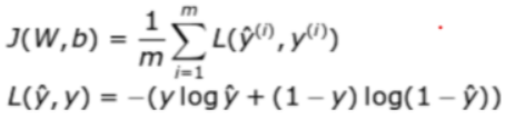
我们计划将神经网络应用于二元分类问题，即模型最后的预测结果只有两种情况，对于每个类别我们预测得到的概率将分别为 𝑝 和 1−𝑝。在这个问题中我们将使用交叉熵损失函数 (cross entropy loss)：

在这里插入图片描述

对于二元分类问题，其交叉熵损失函数写作：

在这里插入图片描述

def get_cost_value(Y_hat, Y):
    # number of examples (=900)
    m = Y_hat.shape[1]
    # calculation of the cost according to the formula
    # - Y: each element is either 0 or 1
    # - shape of Y & Y_hat: (1,900)
    # - shape of cost: (1,1)
    cost = -1 / m * (np.dot(Y, np.log(Y_hat).T) + np.dot(1 - Y, np.log(1 - Y_hat).T))
    
    return np.squeeze(cost)  # np.squeeze() -  从数组的形状中删除单维条目，即把shape中为1的维度去掉

为了取得更多关于学习过程的信息，我们还可以另外实现一个计算精确度的函数。

# an auxiliary function that converts probability into class
def convert_prob_into_class(probs):
    probs_ = np.copy(probs)
    probs_[probs_ > 0.5] = 1
    probs_[probs_ <= 0.5] = 0
    return probs_

def get_accuracy_value(Y_hat, Y):
    Y_hat_ = convert_prob_into_class(Y_hat)  # shape: (1,900)
    accuracy = (Y_hat_ == Y).all(axis=0).mean()  # numpy.all(): 测试沿给定轴的所有数组元素是否都计算为True
                                                 # (Y_hat_ == Y).all(axis=0).shape = (900,)
                                                 # numpy.mean(): 求取均值
    return accuracy

8. 实现神经网络的反向传播过程

和前向传播一样，我们将把网络的反向传播过程拆分成两个函数来实现：

函数 8-1 (single_layer_backward_propagation)：实现单个全连接层的反向传播过程
函数 8-2 (full_backward_propagation)：基于函数 8-1，实现整个神经网络的反向传播过程

8.1　函数 8-1 (single_layer_backward_propagation)：实现单个全连接层的反向传播过程

下图显示了单个神经元上的前向传播和反向传播过程。对一个神经网络层 (𝑙)，我们将接收传输自 𝑙+1 层的 𝑑𝐴[𝑙]，并根据前向传播时保存在 𝑚𝑒𝑚𝑜𝑟𝑦 的中间数据 𝑍_𝑐𝑢𝑟𝑟 和 𝐴_𝑝𝑟𝑒𝑣，计算 𝑙𝑜𝑠𝑠对权重 𝑊[𝑙]和偏置 𝑏[𝑙]的偏导数——𝑑𝑊[𝑙]和 𝑑𝑏[𝑙]。

下面的公式描述了单个全连接层上的反向传播过程。由于本次实验的重点在于实际实现，所以此处省略求导过程，感兴趣的同学请阅读课本相关章节。从公式上我们可以很明显地看到，为什么之前需要在前向传播时记住中间层的 𝐴_𝑝𝑟𝑒𝑣 和 𝑍_𝑐𝑢𝑟𝑟 矩阵的值。

在这里插入图片描述

def single_layer_backward_propagation(dA_curr, W_curr, b_curr, Z_curr, A_prev, activation="relu"):
    # number of examples
    m = A_prev.shape[1]
    
    # selection of activation function
    if activation is "relu":
        backward_activation_func = relu_backward
    elif activation is "sigmoid":
        backward_activation_func = sigmoid_backward
    else:
        raise Exception('Non-supported activation function')

    # step-1: {dA_curr, Z_curr} -> dZ_curr (activation function derivative)
    dZ_curr = backward_activation_func(dA_curr, Z_curr)
    
    
    # step-2: {dZ_curr, A_prev} -> dW_curr (derivative of the matrix W)
    #         dZ_curr -> db_curr (derivative of the vector b)
    
    ###############  Please finish this part  ################
    
    # [Hint]: get dW_curr and db_curr from dZ_curr and A_prev
    #   dW_curr = np.dot(XXX，XXX) / m
    
    dW_curr = np.dot(dZ_curr, A_prev.T) / m

    ########################  end  ###########################
    
    db_curr = np.sum(dZ_curr, axis=1, keepdims=True) / m  # np.sum(): sum of array elements over a given axis
    # or, you can write it as:
    # db_curr = np.dot(dZ_curr, np.ones((dZ_curr.shape[1], 1))) / m  # dZ_curr.shape[1] = 900
    
    
    # step-3: {dZ_curr, W_curr} -> dA_prev (derivative of the matrix A_prev)
    
    ###############  Please finish this part  ################

    # [Hint]: get dA_prev from dZ_curr and W_curr
    #   dA_prev = np.dot(XXX，XXX)
    
    dA_prev = np.dot(W_curr.T, dZ_curr)
    
    ########################  end  ###########################

    return dA_prev, dW_curr, db_curr

代码解释：根据公式可知，矩阵dW_curr的微分是(dZl*A[l-1]T)/m，不难发现dZl正是向量dZ_curr，而A[l-1]T则是向量A_prev的转置。向量dA_prev是 WlTdZl*，WlT是向量W_curr的转置，dZ*l是向量dZ_curr。

8.2　函数 8-2 (full_backward_propagation)：实现整个神经网络的反向传播过程

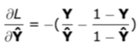
基于单个网络层的反向传播函数，我们从最后一层开始迭代计算所有参数上的导数（𝑑𝑊 和 𝑑𝑏），并最终返回包含所需梯度的字典。为了计算各层参数上的导数，函数需要输入前向传播时的网络输出 𝑌_ℎ𝑎𝑡 和标准结果 𝑌，并交由损失函数计算 𝑙𝑜𝑠𝑠。𝑙𝑜𝑠𝑠对于 𝑌_ℎ𝑎𝑡 的偏导数可计算如下：

在这里插入图片描述

此外，函数还需要输入如下信息：

前向传播时的中间数据 𝑚𝑒𝑚𝑜𝑟𝑦(含 𝐴_𝑝𝑟𝑒𝑣 和 𝑍_𝑐𝑢𝑟𝑟) —— 用以计算各层的 𝑑𝑊 和 𝑑𝑏；
神经网络的参数 𝑝𝑎𝑟𝑎𝑚𝑠_𝑣𝑎𝑙𝑢𝑒𝑠 —— 用以计算各层的 𝑑𝐴_𝑝𝑟𝑒𝑣。

函数的输出是各层的 𝑑𝑊 和 𝑑𝑏，保存在 𝑔𝑟𝑎𝑑𝑠_𝑣𝑎𝑙𝑢𝑒𝑠 中。

在编写函数8-2前，我们先来试验一下等下将怎样从最后一层开始，向前逐层处理网络：

# let's see how we will access each layer in the backward pass
for layer_idx_prev, layer in reversed(list(enumerate(NN_ARCHITECTURE))):  # we will use this code line in the function 8-2
    print(layer_idx_prev)  # from 4 to 0
    print(layer)  # from layer L to layer 1 (we number network layers from 1)

4
{'input_dim': 25, 'output_dim': 1, 'activation': 'sigmoid'}
3
{'input_dim': 50, 'output_dim': 25, 'activation': 'relu'}
2
{'input_dim': 50, 'output_dim': 50, 'activation': 'relu'}
1
{'input_dim': 25, 'output_dim': 50, 'activation': 'relu'}
0
{'input_dim': 2, 'output_dim': 25, 'activation': 'relu'}

def full_backward_propagation(Y_hat, Y, memory, params_values, nn_architecture):
    grads_values = {}
    
    # number of examples (Y.shape=(1,900))
    m = Y.shape[1]
    # a hack ensuring the same shape of the prediction vector and labels vector
    Y = Y.reshape(Y_hat.shape)
    
    # initiation of gradient descent algorithm
    dA_prev = - (np.divide(Y, Y_hat) - np.divide(1 - Y, 1 - Y_hat));
    
    for layer_idx_prev, layer in reversed(list(enumerate(nn_architecture))):
        # we number network layers from 1
        layer_idx_curr = layer_idx_prev + 1
        # extraction of the activation function for the current layer
        activ_function_curr = layer["activation"]
        
        dA_curr = dA_prev
        
        A_prev = memory["A" + str(layer_idx_prev)]
        Z_curr = memory["Z" + str(layer_idx_curr)]
        
        W_curr = params_values["W" + str(layer_idx_curr)]
        b_curr = params_values["b" + str(layer_idx_curr)]
        
        dA_prev, dW_curr, db_curr = single_layer_backward_propagation(
            dA_curr, W_curr, b_curr, Z_curr, A_prev, activ_function_curr)
        
        grads_values["dW" + str(layer_idx_curr)] = dW_curr
        grads_values["db" + str(layer_idx_curr)] = db_curr
    
    return grads_values

9. 更新参数值

反向传播是为了计算梯度，以根据梯度进行优化，更新网络的参数值。为了完成这一任务，我们将使用如下两组数据：

𝑝𝑎𝑟𝑎𝑚𝑠_𝑣𝑎𝑙𝑢𝑒𝑠，其中保存了当前参数值；
𝑔𝑟𝑎𝑑𝑠_𝑣𝑎𝑙𝑢𝑒𝑠，其中保存了用于更新参数值所需的梯度信息。

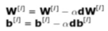
接下来我们只需在每个网络层上应用以下公式即可。其中，𝛼 指学习率 (learning rate)。

在这里插入图片描述

def update(params_values, grads_values, nn_architecture, learning_rate):
    # iteration over network layers
    for idx, layer in enumerate(nn_architecture):
        layer_idx = idx + 1
        
        ###############  Please finish this part  ################
        
        # [Hint]: update params_values
        #   params_values["W" + str(layer_idx)] = XXX
        #   params_values["b" + str(layer_idx)] = XXX

        params_values["W" + str(layer_idx)] -= learning_rate * grads_values["dW" + str(layer_idx)]
        params_values["b" + str(layer_idx)] -= learning_rate * grads_values["db" + str(layer_idx)]
        
        ########################  end  ###########################

    return params_values

代码解释：每一层的权重矩阵 𝑊 和偏置向量 𝑏均以Wl与bl的形式保存在params_values中，而grads_values中保存了用于更新参数值所需的梯度信息。根据已经给出的公式可知，参数的更新是每次减去梯度乘以学习率，据此可以填写代码。

10. 整合：完成 train 函数

到目前为止，我们已经完成了最困难的部分，准备好了所需的函数，接下来只需以正确的顺序把它们整合到一起。为了更好地理解每一步操作的顺序，请同学们再次查看“0. 概览”中的训练流程图。

train 函数将返回经过训练优化后的参数值，并显示在训练期间模型在训练集上的准确率。后期在测试集上，只需使用训练好的模型参数并运行一次完整的前向传播过程即可。

def train(X, Y, nn_architecture, epochs, learning_rate, verbose=True, callback=None):
    # initiation of neural net parameters
    params_values = init_layers(nn_architecture, 2)
    # initiation of lists storing the history of metrics calculated during the learning process 
    cost_history = []
    accuracy_history = []
    
    # performing calculations for subsequent iterations
    for i in range(epochs):
        # step forward
        Y_hat, cache = full_forward_propagation(X, params_values, nn_architecture)
        
        if i==1:
            print("X.shape: ", X.shape)  # (2, 900)
            print("Y_hat.shape: ", Y_hat.shape)  # (1, 900)
            print("Y.shape: ", Y.shape)  # (1, 900)
        
        # calculating metrics and saving them in history
        cost = get_cost_value(Y_hat, Y)
        cost_history.append(cost)
        accuracy = get_accuracy_value(Y_hat, Y)
        accuracy_history.append(accuracy)
        
        # step backward - calculating gradient
        grads_values = full_backward_propagation(Y_hat, Y, cache, params_values, nn_architecture)
        # updating model state
        params_values = update(params_values, grads_values, nn_architecture, learning_rate)
        
        if(i % 50 == 0):
            if(verbose):
                print("Iteration: {:05} - cost: {:.5f} - accuracy: {:.5f}".format(i, cost, accuracy))
            if(callback is not None):
                callback(i, params_values)
            
    return params_values

11. 数据集准备

现在是时候尝试应用我们的模型来解决一个简单的分类问题。为了检测模型是否能够顺利训练，下面我们将生成一个含有两个类的点集（如下图所示，两个类别的点分别用不同颜色表示），然后尝试训练模型来对这些点进行分类（二元分类问题）。

在这里插入图片描述

# number of samples in the data set
N_SAMPLES = 1000
# ratio between training and test sets
TEST_SIZE = 0.1

# we will use sklearn.make_moons() to generate the dataset:
#  - n_samples: 生成样本数量
#  - noise: 高斯噪声
#  - random_state: 生成随机种子，给定一个int型数据，能够保证每次生成数据相同
X, y = make_moons(n_samples = N_SAMPLES, noise=0.2, random_state=100)

# split the dataset into training set (90%) & test set (10%)
#  - test_size: 如果是浮点数，则应该在0.0和1.0之间，表示要测试集占总数据集的比例；如果是int类型，表示测试集的绝对数量。
#  - random_state: 随机数生成器使用的种子
X_train, X_test, y_train, y_test = train_test_split(X, y, test_size=TEST_SIZE, random_state=42)

下面我们来观察一下刚刚生成好的数据集。

shape of X:  (1000, 2)
X =  [[ 2.24907069e-05  1.07275825e+00]
 [-5.59037377e-02  4.25241282e-01]
 [ 2.40944879e-02  4.08065802e-01]
 ...
 [ 1.75841594e+00 -5.77404262e-01]
 [ 1.26710180e+00 -4.42980152e-01]
 [-1.75927072e-01  5.83509936e-01]]
shape of X:  (900, 2)

# check the information in Y
print("shape of Y: ", y.shape)  # (1000,)
print("number of zeros in Y: ", np.sum(y==0))  # 500
print("number of ones in Y: ", np.sum(y==1))  # 500
print("Y = ", y)

shape of Y:  (1000,)
number of zeros in Y:  500
number of ones in Y:  500
Y =  [0 0 1 0 1 0 0 1 1 1 1 1 0 1 1 0 0 1 0 1 1 0 1 0 0 1 1 0 1 1 1 0 0 0 0 1 1
 1 0 0 0 0 0 0 1 0 1 0 1 0 0 1 0 0 0 0 1 1 1 0 0 1 1 0 1 0 0 0 0 0 1 1 1 0
 1 0 0 1 0 1 1 1 1 0 1 0 1 1 0 1 0 0 1 0 0 1 0 0 0 0 1 1 0 1 1 0 0 0 1 0 0
 0 0 1 1 0 0 0 1 0 1 1 0 0 1 1 0 0 1 1 0 0 1 0 0 0 1 0 0 1 1 0 0 0 1 0 0 0
 0 1 0 1 1 1 1 0 1 1 1 0 1 1 0 0 1 0 1 0 1 1 0 0 1 0 1 0 0 1 1 1 1 1 0 1 1
 0 0 0 0 0 1 0 1 0 1 1 1 0 0 1 1 0 0 1 1 1 0 0 1 1 0 0 0 0 0 0 0 0 0 1 0 0
 1 1 0 1 0 0 1 1 0 1 0 0 0 0 1 1 1 1 0 0 0 0 0 1 0 0 1 1 1 0 1 1 1 1 1 1 1
 0 0 0 0 0 0 1 1 1 1 0 1 0 0 0 1 1 1 0 0 1 0 1 1 1 0 0 1 0 0 0 1 1 0 1 0 0
 1 1 0 0 0 0 0 0 1 0 0 0 1 0 1 0 0 1 0 1 1 1 0 0 1 0 1 0 1 0 1 0 0 1 0 1 1
 0 0 1 0 1 1 0 0 1 1 1 1 0 0 1 1 0 1 1 0 1 1 0 1 1 0 0 1 0 0 1 0 0 0 1 1 0
 0 1 1 1 1 0 0 0 0 1 0 0 0 0 1 1 0 1 1 1 0 0 1 0 1 0 1 1 0 0 1 0 1 1 1 1 0
 1 0 0 0 0 1 0 0 0 0 0 0 1 1 1 1 0 1 0 1 1 1 1 0 1 1 1 1 0 1 0 0 1 1 1 1 0
 1 1 1 0 1 1 1 1 1 0 1 1 1 0 0 1 0 1 0 0 0 1 1 1 0 0 0 0 1 1 1 0 1 0 1 0 0
 1 0 1 0 1 1 0 1 0 0 0 1 1 1 1 0 1 1 0 0 1 1 0 0 0 1 0 0 0 0 1 0 1 1 0 1 1
 1 0 0 1 0 0 0 0 0 1 1 1 1 0 1 0 1 1 0 0 0 0 0 1 0 0 0 0 1 1 1 1 0 1 1 0 0
 0 1 1 0 1 1 0 1 0 1 1 0 1 0 0 0 0 1 1 0 0 0 1 1 1 0 1 0 1 1 1 1 0 1 1 1 1
 0 1 1 0 0 1 1 1 1 1 0 0 0 0 0 1 1 0 0 1 0 1 1 1 1 0 0 1 0 0 0 0 0 0 0 0 0
 1 0 0 1 0 1 1 0 1 1 0 1 1 0 1 0 1 0 1 0 1 0 1 0 1 1 1 0 0 1 1 1 0 1 1 0 1
 0 1 0 1 1 0 1 1 1 0 1 1 0 1 0 1 1 1 0 1 1 0 1 0 1 0 0 0 0 1 1 1 0 1 1 1 0
 1 1 0 0 1 0 0 1 1 1 0 1 1 0 0 0 1 1 0 1 0 0 1 0 0 1 0 0 1 1 1 1 1 1 1 0 1
 0 0 1 1 1 1 0 0 1 0 0 0 0 1 1 1 0 1 0 0 0 0 1 0 1 1 1 1 1 1 0 0 1 1 0 1 0
 1 0 1 1 0 0 1 1 1 0 1 1 0 1 0 0 1 0 1 1 1 1 1 1 0 0 1 0 0 0 0 0 1 0 1 0 0
 0 0 0 1 1 1 1 1 0 0 0 1 1 0 1 0 1 0 1 0 1 0 0 0 1 0 1 0 1 0 0 0 1 1 0 0 1
 0 1 1 1 0 0 1 0 1 0 0 0 1 0 1 1 0 0 0 1 0 0 1 0 1 1 0 0 0 0 1 0 1 1 1 0 1
 0 1 0 0 0 1 1 0 1 0 0 1 1 0 1 0 0 1 0 1 1 0 0 0 0 0 0 1 1 0 0 0 0 1 0 0 1
 1 1 0 1 0 0 0 0 1 1 1 0 1 0 0 1 0 0 0 0 0 1 1 0 0 1 1 1 0 1 0 0 0 1 1 1 0
 1 1 1 0 1 0 1 1 1 0 0 0 1 1 1 1 0 1 0 1 0 1 1 1 1 1 0 1 1 0 1 1 0 1 1 1 1
 1]

# the function making up the graph of a dataset
def make_plot(X, y, plot_name, file_name=None, XX=None, YY=None, preds=None, dark=False):
    if (dark):
        plt.style.use('dark_background')
    else:
        sns.set_style("whitegrid")
    plt.figure(figsize=(16,12))
    axes = plt.gca()
    axes.set(xlabel="$X_1$", ylabel="$X_2$")
    plt.title(plot_name, fontsize=30)
    plt.subplots_adjust(left=0.20)
    plt.subplots_adjust(right=0.80)
    if(XX is not None and YY is not None and preds is not None):
        plt.contourf(XX, YY, preds.reshape(XX.shape), 25, alpha = 1, cmap=cm.Spectral)
        plt.contour(XX, YY, preds.reshape(XX.shape), levels=[.5], cmap="Greys", vmin=0, vmax=.6)
    plt.scatter(X[:, 0], X[:, 1], c=y.ravel(), s=40, cmap=plt.cm.Spectral, edgecolors='black')
    if(file_name):
        plt.savefig(file_name)
        plt.close()

# plot the dataset
make_plot(X, y, "Dataset")

在这里插入图片描述

请同学们依次尝试将 sklearn.make_moons() 函数中 noise 取 0, 0.2, 0.4, 0.8, 1.0 等不同值，查看并截图保存对应的数据集图像和训练结果，分析其趋势，及出现这样趋势的原因。

然后，请同学们将 sklearn.make_moons() 中 noise 固定为 0.8，将sklearn.model_selection.train_test_split() 函数中的 TEST_SIZE 改为 0.98，观察和原先 noise 为 0.2、TEST_SIZE 为 0.1 的情况相比，训练集上的准确度和测试集上的准确度都分别发生了什么变化？出现这样变化的原因是什么？

调整 make_moons() 函数中的 noise 和 train_test_split() 函数中的 TEST_SIZE，改变数据集中点的分布。将 sklearn.make_moons() 中 noise 固定为 0.8，将sklearn.model_selection.train_test_split() 函数中的 TEST_SIZE 改为 0.98，观察和原先 noise 为 0.2、TEST_SIZE 为 0.1 的情况相比，训练过程折线图表示如图所示，测试结果如图所示。

在这里插入图片描述

结论：当测试集占总数据量10%，noise等于0.2时，训练速度较慢，但是Acc和Cost曲线比较平滑，且测试效果和模型最终在训练集上得到的效果相差不大，即可以学习出一种较好的模型。而当测试集占总数据量98%，noise等于0.8时，训练速度较快，但是Acc曲线出现毛刺，且测试效果和模型最终在训练集上得到的效果很大，即出现过拟合现象。分析可知，当训练集占比过小，模型只能学习到很少的知识，无法得到好的模型。

12. 模型训练及测试

下面我们来调用 train 函数对模型进行训练。

# let's train the neural network
params_values = train(X=np.transpose(X_train), Y=np.transpose(y_train.reshape((y_train.shape[0], 1))), 
                      nn_architecture=NN_ARCHITECTURE, epochs=10000, learning_rate=0.01)

Iteration: 00000 - cost: 0.69365 - accuracy: 0.50444
X.shape:  (2, 900)
Y_hat.shape:  (1, 900)
Y.shape:  (1, 900)
Iteration: 00050 - cost: 0.69349 - accuracy: 0.50444
Iteration: 00100 - cost: 0.69334 - accuracy: 0.50444
Iteration: 00150 - cost: 0.69319 - accuracy: 0.50444
Iteration: 00200 - cost: 0.69307 - accuracy: 0.50444
Iteration: 00250 - cost: 0.69295 - accuracy: 0.50444
Iteration: 00300 - cost: 0.69284 - accuracy: 0.50444
Iteration: 00350 - cost: 0.69272 - accuracy: 0.50444
Iteration: 00400 - cost: 0.69260 - accuracy: 0.50444
Iteration: 00450 - cost: 0.69249 - accuracy: 0.50444
Iteration: 00500 - cost: 0.69238 - accuracy: 0.50444
Iteration: 00550 - cost: 0.69228 - accuracy: 0.50444
Iteration: 00600 - cost: 0.69217 - accuracy: 0.50444
Iteration: 00650 - cost: 0.69206 - accuracy: 0.50444
Iteration: 00700 - cost: 0.69194 - accuracy: 0.50444
Iteration: 00750 - cost: 0.69182 - accuracy: 0.50444
Iteration: 00800 - cost: 0.69170 - accuracy: 0.50444
Iteration: 00850 - cost: 0.69156 - accuracy: 0.50444
Iteration: 00900 - cost: 0.69142 - accuracy: 0.50444
Iteration: 00950 - cost: 0.69126 - accuracy: 0.50444
Iteration: 01000 - cost: 0.69109 - accuracy: 0.50444
Iteration: 01050 - cost: 0.69090 - accuracy: 0.50444
Iteration: 01100 - cost: 0.69070 - accuracy: 0.50444
Iteration: 01150 - cost: 0.69049 - accuracy: 0.50444
Iteration: 01200 - cost: 0.69025 - accuracy: 0.50444
Iteration: 01250 - cost: 0.69000 - accuracy: 0.50889
Iteration: 01300 - cost: 0.68972 - accuracy: 0.52889
Iteration: 01350 - cost: 0.68941 - accuracy: 0.59778
Iteration: 01400 - cost: 0.68907 - accuracy: 0.66667
Iteration: 01450 - cost: 0.68869 - accuracy: 0.72222
Iteration: 01500 - cost: 0.68827 - accuracy: 0.76111
Iteration: 01550 - cost: 0.68780 - accuracy: 0.79111
Iteration: 01600 - cost: 0.68726 - accuracy: 0.81333
Iteration: 01650 - cost: 0.68666 - accuracy: 0.82778
Iteration: 01700 - cost: 0.68596 - accuracy: 0.83778
Iteration: 01750 - cost: 0.68512 - accuracy: 0.84000
Iteration: 01800 - cost: 0.68416 - accuracy: 0.84222
Iteration: 01850 - cost: 0.68308 - accuracy: 0.84444
Iteration: 01900 - cost: 0.68185 - accuracy: 0.84333
Iteration: 01950 - cost: 0.68042 - accuracy: 0.84222
Iteration: 02000 - cost: 0.67875 - accuracy: 0.84222
Iteration: 02050 - cost: 0.67680 - accuracy: 0.84444
Iteration: 02100 - cost: 0.67453 - accuracy: 0.84444
Iteration: 02150 - cost: 0.67183 - accuracy: 0.84667
Iteration: 02200 - cost: 0.66859 - accuracy: 0.84556
Iteration: 02250 - cost: 0.66471 - accuracy: 0.84222
Iteration: 02300 - cost: 0.66004 - accuracy: 0.84333
Iteration: 02350 - cost: 0.65437 - accuracy: 0.84222
Iteration: 02400 - cost: 0.64757 - accuracy: 0.84444
Iteration: 02450 - cost: 0.63942 - accuracy: 0.84778
Iteration: 02500 - cost: 0.62966 - accuracy: 0.84444
Iteration: 02550 - cost: 0.61796 - accuracy: 0.84111
Iteration: 02600 - cost: 0.60398 - accuracy: 0.84111
Iteration: 02650 - cost: 0.58764 - accuracy: 0.84111
Iteration: 02700 - cost: 0.56876 - accuracy: 0.84222
Iteration: 02750 - cost: 0.54730 - accuracy: 0.84222
Iteration: 02800 - cost: 0.52368 - accuracy: 0.85000
Iteration: 02850 - cost: 0.49867 - accuracy: 0.85333
Iteration: 02900 - cost: 0.47325 - accuracy: 0.85556
Iteration: 02950 - cost: 0.44840 - accuracy: 0.85556
Iteration: 03000 - cost: 0.42476 - accuracy: 0.85889
Iteration: 03050 - cost: 0.40263 - accuracy: 0.86333
Iteration: 03100 - cost: 0.38221 - accuracy: 0.86222
Iteration: 03150 - cost: 0.36367 - accuracy: 0.86778
Iteration: 03200 - cost: 0.34730 - accuracy: 0.87111
Iteration: 03250 - cost: 0.33327 - accuracy: 0.87444
Iteration: 03300 - cost: 0.32149 - accuracy: 0.87778
Iteration: 03350 - cost: 0.31175 - accuracy: 0.87889
Iteration: 03400 - cost: 0.30379 - accuracy: 0.88000
Iteration: 03450 - cost: 0.29733 - accuracy: 0.88111
Iteration: 03500 - cost: 0.29209 - accuracy: 0.88111
Iteration: 03550 - cost: 0.28783 - accuracy: 0.88111
Iteration: 03600 - cost: 0.28431 - accuracy: 0.88222
Iteration: 03650 - cost: 0.28133 - accuracy: 0.88333
Iteration: 03700 - cost: 0.27875 - accuracy: 0.88333
Iteration: 03750 - cost: 0.27648 - accuracy: 0.88333
Iteration: 03800 - cost: 0.27445 - accuracy: 0.88333
Iteration: 03850 - cost: 0.27262 - accuracy: 0.88222
Iteration: 03900 - cost: 0.27090 - accuracy: 0.88111
Iteration: 03950 - cost: 0.26930 - accuracy: 0.88000
Iteration: 04000 - cost: 0.26780 - accuracy: 0.88000
Iteration: 04050 - cost: 0.26634 - accuracy: 0.88000
Iteration: 04100 - cost: 0.26495 - accuracy: 0.88000
Iteration: 04150 - cost: 0.26356 - accuracy: 0.88000
Iteration: 04200 - cost: 0.26215 - accuracy: 0.87889
Iteration: 04250 - cost: 0.26074 - accuracy: 0.88000
Iteration: 04300 - cost: 0.25933 - accuracy: 0.88222
Iteration: 04350 - cost: 0.25793 - accuracy: 0.88333
Iteration: 04400 - cost: 0.25652 - accuracy: 0.88444
Iteration: 04450 - cost: 0.25510 - accuracy: 0.88444
Iteration: 04500 - cost: 0.25369 - accuracy: 0.88444
Iteration: 04550 - cost: 0.25227 - accuracy: 0.88333
Iteration: 04600 - cost: 0.25087 - accuracy: 0.88444
Iteration: 04650 - cost: 0.24944 - accuracy: 0.88556
Iteration: 04700 - cost: 0.24798 - accuracy: 0.88556
Iteration: 04750 - cost: 0.24650 - accuracy: 0.88667
Iteration: 04800 - cost: 0.24497 - accuracy: 0.88778
Iteration: 04850 - cost: 0.24336 - accuracy: 0.88778
Iteration: 04900 - cost: 0.24171 - accuracy: 0.88889
Iteration: 04950 - cost: 0.23999 - accuracy: 0.89000
Iteration: 05000 - cost: 0.23821 - accuracy: 0.89000
Iteration: 05050 - cost: 0.23635 - accuracy: 0.89222
Iteration: 05100 - cost: 0.23441 - accuracy: 0.89333
Iteration: 05150 - cost: 0.23237 - accuracy: 0.89333
Iteration: 05200 - cost: 0.23021 - accuracy: 0.89444
Iteration: 05250 - cost: 0.22792 - accuracy: 0.89556
Iteration: 05300 - cost: 0.22550 - accuracy: 0.89667
Iteration: 05350 - cost: 0.22292 - accuracy: 0.89667
Iteration: 05400 - cost: 0.22018 - accuracy: 0.89778
Iteration: 05450 - cost: 0.21728 - accuracy: 0.90000
Iteration: 05500 - cost: 0.21418 - accuracy: 0.90222
Iteration: 05550 - cost: 0.21087 - accuracy: 0.90444
Iteration: 05600 - cost: 0.20736 - accuracy: 0.90556
Iteration: 05650 - cost: 0.20364 - accuracy: 0.91111
Iteration: 05700 - cost: 0.19973 - accuracy: 0.91333
Iteration: 05750 - cost: 0.19562 - accuracy: 0.91444
Iteration: 05800 - cost: 0.19133 - accuracy: 0.91889
Iteration: 05850 - cost: 0.18686 - accuracy: 0.92222
Iteration: 05900 - cost: 0.18224 - accuracy: 0.92556
Iteration: 05950 - cost: 0.17747 - accuracy: 0.92778
Iteration: 06000 - cost: 0.17260 - accuracy: 0.93000
Iteration: 06050 - cost: 0.16767 - accuracy: 0.93333
Iteration: 06100 - cost: 0.16269 - accuracy: 0.93444
Iteration: 06150 - cost: 0.15775 - accuracy: 0.93778
Iteration: 06200 - cost: 0.15289 - accuracy: 0.93778
Iteration: 06250 - cost: 0.14812 - accuracy: 0.93889
Iteration: 06300 - cost: 0.14350 - accuracy: 0.94333
Iteration: 06350 - cost: 0.13907 - accuracy: 0.94444
Iteration: 06400 - cost: 0.13485 - accuracy: 0.94444
Iteration: 06450 - cost: 0.13086 - accuracy: 0.94556
Iteration: 06500 - cost: 0.12711 - accuracy: 0.94667
Iteration: 06550 - cost: 0.12361 - accuracy: 0.95000
Iteration: 06600 - cost: 0.12035 - accuracy: 0.95444
Iteration: 06650 - cost: 0.11733 - accuracy: 0.95778
Iteration: 06700 - cost: 0.11456 - accuracy: 0.95778
Iteration: 06750 - cost: 0.11200 - accuracy: 0.95889
Iteration: 06800 - cost: 0.10963 - accuracy: 0.96000
Iteration: 06850 - cost: 0.10745 - accuracy: 0.96000
Iteration: 06900 - cost: 0.10544 - accuracy: 0.96222
Iteration: 06950 - cost: 0.10359 - accuracy: 0.96111
Iteration: 07000 - cost: 0.10188 - accuracy: 0.96111
Iteration: 07050 - cost: 0.10031 - accuracy: 0.96222
Iteration: 07100 - cost: 0.09885 - accuracy: 0.96222
Iteration: 07150 - cost: 0.09750 - accuracy: 0.96222
Iteration: 07200 - cost: 0.09623 - accuracy: 0.96222
Iteration: 07250 - cost: 0.09506 - accuracy: 0.96444
Iteration: 07300 - cost: 0.09399 - accuracy: 0.96556
Iteration: 07350 - cost: 0.09298 - accuracy: 0.96556
Iteration: 07400 - cost: 0.09203 - accuracy: 0.96667
Iteration: 07450 - cost: 0.09118 - accuracy: 0.96667
Iteration: 07500 - cost: 0.09041 - accuracy: 0.96667
Iteration: 07550 - cost: 0.08969 - accuracy: 0.96667
Iteration: 07600 - cost: 0.08898 - accuracy: 0.96667
Iteration: 07650 - cost: 0.08831 - accuracy: 0.96667
Iteration: 07700 - cost: 0.08767 - accuracy: 0.96667
Iteration: 07750 - cost: 0.08707 - accuracy: 0.96667
Iteration: 07800 - cost: 0.08647 - accuracy: 0.96778
Iteration: 07850 - cost: 0.08594 - accuracy: 0.96667
Iteration: 07900 - cost: 0.08544 - accuracy: 0.96667
Iteration: 07950 - cost: 0.08497 - accuracy: 0.96667
Iteration: 08000 - cost: 0.08453 - accuracy: 0.96556
Iteration: 08050 - cost: 0.08412 - accuracy: 0.96667
Iteration: 08100 - cost: 0.08371 - accuracy: 0.96667
Iteration: 08150 - cost: 0.08332 - accuracy: 0.96889
Iteration: 08200 - cost: 0.08295 - accuracy: 0.96889
Iteration: 08250 - cost: 0.08259 - accuracy: 0.96889
Iteration: 08300 - cost: 0.08219 - accuracy: 0.96889
Iteration: 08350 - cost: 0.08180 - accuracy: 0.96778
Iteration: 08400 - cost: 0.08145 - accuracy: 0.96778
Iteration: 08450 - cost: 0.08114 - accuracy: 0.96778
Iteration: 08500 - cost: 0.08084 - accuracy: 0.96889
Iteration: 08550 - cost: 0.08055 - accuracy: 0.96889
Iteration: 08600 - cost: 0.08025 - accuracy: 0.97000
Iteration: 08650 - cost: 0.07996 - accuracy: 0.97000
Iteration: 08700 - cost: 0.07968 - accuracy: 0.97000
Iteration: 08750 - cost: 0.07939 - accuracy: 0.97000
Iteration: 08800 - cost: 0.07912 - accuracy: 0.96889
Iteration: 08850 - cost: 0.07885 - accuracy: 0.96889
Iteration: 08900 - cost: 0.07860 - accuracy: 0.96889
Iteration: 08950 - cost: 0.07836 - accuracy: 0.96889
Iteration: 09000 - cost: 0.07812 - accuracy: 0.96889
Iteration: 09050 - cost: 0.07788 - accuracy: 0.96889
Iteration: 09100 - cost: 0.07765 - accuracy: 0.96889
Iteration: 09150 - cost: 0.07743 - accuracy: 0.96889
Iteration: 09200 - cost: 0.07721 - accuracy: 0.96889
Iteration: 09250 - cost: 0.07698 - accuracy: 0.96889
Iteration: 09300 - cost: 0.07676 - accuracy: 0.96889
Iteration: 09350 - cost: 0.07653 - accuracy: 0.96889
Iteration: 09400 - cost: 0.07631 - accuracy: 0.96889
Iteration: 09450 - cost: 0.07610 - accuracy: 0.96889
Iteration: 09500 - cost: 0.07588 - accuracy: 0.96889
Iteration: 09550 - cost: 0.07568 - accuracy: 0.96889
Iteration: 09600 - cost: 0.07550 - accuracy: 0.96889
Iteration: 09650 - cost: 0.07532 - accuracy: 0.96889
Iteration: 09700 - cost: 0.07516 - accuracy: 0.96889
Iteration: 09750 - cost: 0.07500 - accuracy: 0.96889
Iteration: 09800 - cost: 0.07485 - accuracy: 0.96889
Iteration: 09850 - cost: 0.07470 - accuracy: 0.96889
Iteration: 09900 - cost: 0.07456 - accuracy: 0.96889
Iteration: 09950 - cost: 0.07442 - accuracy: 0.96889

调用一次 full_forward_propagation()，在测试集上评估训练好的模型。

# prediction
Y_test_hat, _ = full_forward_propagation(np.transpose(X_test), params_values, NN_ARCHITECTURE)

# accuracy achieved on the test set
acc_test = get_accuracy_value(Y_test_hat, np.transpose(y_test.reshape((y_test.shape[0], 1))))
print("Test set accuracy: {:.2f}".format(acc_test))