信号处理--基于EEG脑电信号的深度学习情绪分类

本文为一个信号处理专题的课程项目，主要是基于人体脑电信号，通过使用深度学习，来快速精准的识别被试的情绪。实验数据为私有数据集。情绪分为积极，中性，消极三种类别。该方法最后和传统朴素贝叶斯，支持向量机，logistic回归，决策树和随机森林分类器进行比较。

目录

1 加载主要库函数

2 检查eeg脑电信号和数据预处理

2.1 绘制不同种类数据大小比例分布图

2.2 显示积极情绪的脑电信号

2.3 显示消极情绪的脑电信号

 2.4 显示中性情绪的脑电信号

 2.5 数据的预处理

3 搭建LSTM深度学习模型

3.1 定义模型的构建函数

3.2 构建模型

3.3 模型训练和测试

 3.4 使用confusion matrix 评估模型

4 和其他传统模型性能比较

5 绘制模型训练loss和准确率

6 数据集下载

---

---

1 加载主要库函数

import numpy as np # linear algebra
import pandas as pd # data processing, CSV file I/O (e.g. pd.read_csv)
import seaborn as sns
import matplotlib.pyplot as plt
from sklearn.preprocessing import StandardScaler
import tensorflow 
from sklearn.model_selection import train_test_split
from tensorflow.keras.utils import to_categorical
import tensorflow as tf
from tensorflow.keras import Sequential
from tensorflow.keras.optimizers import SGD

from tensorflow.keras.layers import Dense, Dropout
from tensorflow.keras.layers import Embedding
from tensorflow.keras.layers import LSTM
tf.keras.backend.clear_session()
from sklearn.metrics import plot_confusion_matrix
from sklearn import datasets, tree, linear_model, svm
from sklearn.metrics import confusion_matrix,classification_report
from sklearn.ensemble import RandomForestClassifier
from sklearn.naive_bayes import GaussianNB

from sklearn.metrics import confusion_matrix,classification_report
from sklearn.ensemble import RandomForestClassifier
from sklearn.naive_bayes import GaussianNB
from sklearn.metrics import confusion_matrix

import seaborn as sns

2 检查eeg脑电信号和数据预处理

data = pd.read_csv("../input/eeg-brainwave-dataset-feeling-emotions/emotions.csv")

#Seprarting Positive,Neagtive and Neutral dataframes for plortting
pos = data.loc[data["label"]=="POSITIVE"]
sample_pos = pos.loc[2, 'fft_0_b':'fft_749_b']
neg = data.loc[data["label"]=="NEGATIVE"]
sample_neg = neg.loc[0, 'fft_0_b':'fft_749_b']
neu = data.loc[data["label"]=="NEUTRAL"]
sample_neu = neu.loc[1, 'fft_0_b':'fft_749_b']

2.1 绘制不同种类数据大小比例分布图

#plottintg Dataframe distribution
plt.figure(figsize=(25,7))
plt.title("Data distribution of Emotions")
plt.style.use('fivethirtyeight')
sns.countplot(x='label', data=data)
plt.show()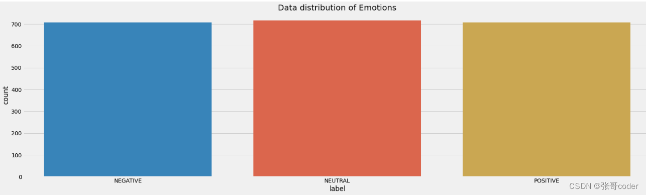

2.2 显示积极情绪的脑电信号

#Plotting Positive DataFrame
plt.figure(figsize=(16, 10))
plt.plot(range(len(sample_pos)), sample_pos)
plt.title("Graph of Positive Columns")
plt.show()
'''As we can noticed the most of the Negative Signals are from greater than 600 to and less than than -600'''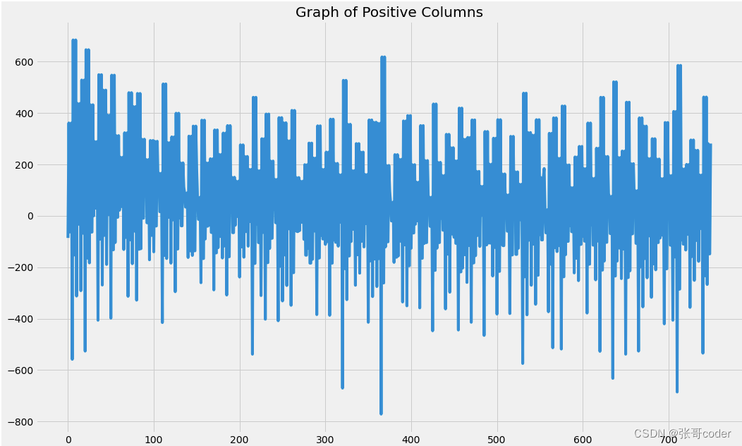

 

2.3 显示消极情绪的脑电信号

#Plotting Negative DataFrame
plt.figure(figsize=(16, 10))
plt.plot(range(len(sample_neg)), sample_neg)
plt.title("Graph of Negative Columns")
plt.show()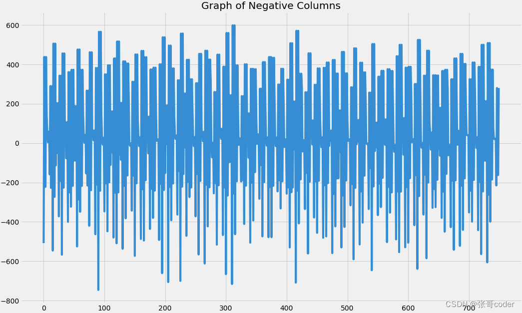

 

 2.4 显示中性情绪的脑电信号

#Plotting Neutral DataFrame
plt.figure(figsize=(16, 10))
plt.plot(range(len(sample_neu)), sample_neu)
plt.title("Graph of Neutral Columns")
plt.show()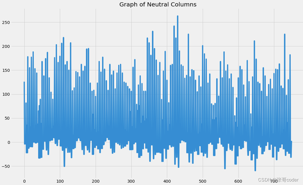

 

 2.5 数据的预处理

def Transform_data(data):
    #Encoding Lables into numbers
    encoding_data = ({'NEUTRAL': 0, 'POSITIVE': 1, 'NEGATIVE': 2} )
    data_encoded = data.replace(encoding_data)
    #getting brain signals into x variable
    x=data_encoded.drop(["label"]  ,axis=1)
    #getting labels into y variable
    y = data_encoded.loc[:,'label'].values
    scaler = StandardScaler()
    #scaling Brain Signals
    scaler.fit(x)
    X = scaler.transform(x)
    #One hot encoding Labels 
    Y = to_categorical(y)
    return X,Y

#Calling above function and splitting dataset into train and test
X,Y = Transform_data(data)
x_train, x_test, y_train, y_test = train_test_split(X, Y, test_size = 0.2, random_state = 4)

3 搭建LSTM深度学习模型

3.1 定义模型的构建函数

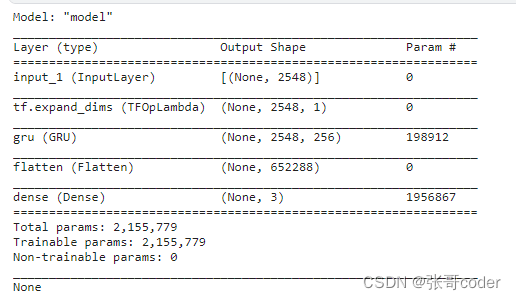
def create_model():
    #input layer of model for brain signals
    inputs = tf.keras.Input(shape=(x_train.shape[1],))
    #Hidden Layer for Brain signal using LSTM(GRU)
    expand_dims = tf.expand_dims(inputs, axis=2)

    gru = tf.keras.layers.GRU(256, return_sequences=True)(expand_dims)
    #Flatten Gru layer into vector form (one Dimensional array)
    flatten = tf.keras.layers.Flatten()(gru)
    #output latyer of Model
    outputs = tf.keras.layers.Dense(3, activation='softmax')(flatten)


    model = tf.keras.Model(inputs=inputs, outputs=outputs)
    print(model.summary())
    return model

3.2 构建模型

#cretaing model
lstmmodel = create_model()
#Compiling model 
lstmmodel.compile(
    optimizer='adam',
    loss='categorical_crossentropy',
    metrics=['accuracy']
)

3.3 模型训练和测试

#Training and Evaluting model
history = lstmmodel.fit(x_train, y_train, epochs = 10, validation_split=0.1)
loss, acc = lstmmodel.evaluate(x_test, y_test)

#Loss and Accuracy of model on Testiong Dataset 
print(f"Loss on testing: {loss*100}",f"\nAccuracy on Training: {acc*100}")

#predicting model on test set for plotting Confusion Matrix
pred  = lstmmodel.predict(x_test)

 3.4 使用confusion matrix 评估模型

#Creation of Function of Confusion Matrix
def plot_confusion_matrix(cm, names, title='Confusion matrix', cmap=plt.cm.Blues):
    plt.imshow(cm, interpolation='nearest', cmap=cmap)
    plt.title(title)
    plt.colorbar()
    tick_marks = np.arange(len(data.label.unique()))
    plt.xticks(tick_marks, names, rotation=90)
    plt.yticks(tick_marks, names)
    plt.tight_layout()
    plt.ylabel('True label')
    plt.xlabel('Predicted label')


#after getting prediction checking maximum score prediction to claim which emotion this brain signal belongs to
pred1 = np.argmax(pred,axis=1)


#inversing the one hot encoding
y_test1 =   np.argmax(y_test,axis=1)



#printing first 10 Actual and predicted outputs of Test brain signals 
print("Predicted:  ",pred1[:10])
print("\n")
print("Actual: ",y_test1[:10])



#Plotting Confusion matrix of Lstm Model
cm = confusion_matrix(y_test1, pred1)
np.set_printoptions(precision=2)
print('Confusion matrix, without normalization')
print(cm)
plt.rcParams["figure.figsize"]=(20,5)
plt.figure()
plot_confusion_matrix(cm,["Neutral","Positive","Negative"])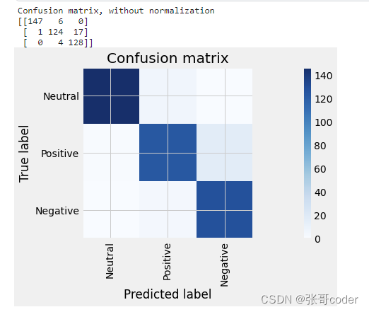

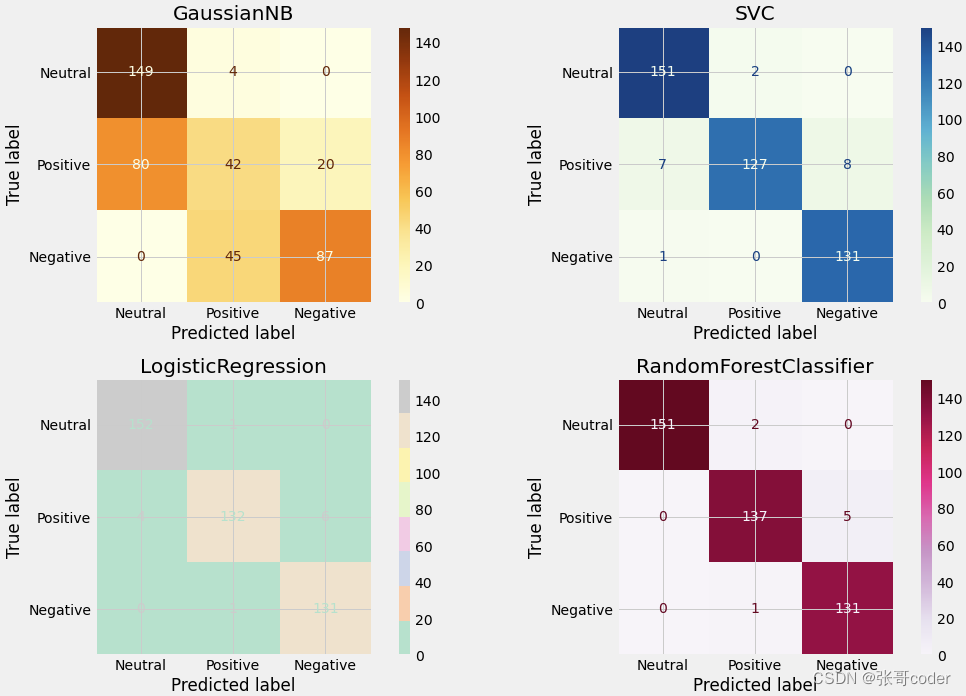
4 和其他传统模型性能比较

names1 = ["Neutral","Positive","Negative"]

#Training our dataset on different Classifiers to check the results and creating their classification reports
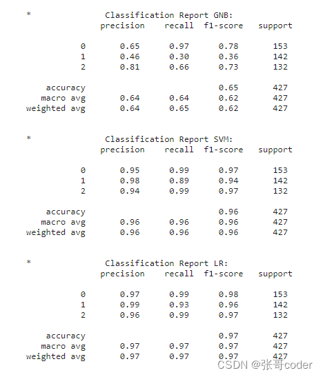
#NAves Bayes Clssifier
Classifier_gnb = GaussianNB().fit(x_train, np.argmax(y_train,axis=1))
pred_gnb = Classifier_gnb.predict(x_test)
print ('\n*\t\tClassification Report GNB:\n', classification_report(np.argmax(y_test,axis=1), pred_gnb))
confusion_matrix_graph = confusion_matrix(np.argmax(y_test,axis=1), pred_gnb)
### Support Vector Machine

Classifier_svm = svm.SVC(kernel='linear').fit(x_train, np.argmax(y_train,axis=1))
pred_svm = Classifier_svm.predict(x_test)
print ('\n*\t\tClassification Report SVM:\n', classification_report(np.argmax(y_test,axis=1), pred_svm))
confusion_matrix_graph = confusion_matrix(np.argmax(y_test,axis=1), pred_svm)
### Logistic Regression

Classifier_LR = linear_model.LogisticRegression(solver = 'liblinear', C = 75).fit(x_train, np.argmax(y_train,axis=1))
pred_LR = Classifier_LR.predict(x_test)
print ('\n*\t\tClassification Report LR:\n', classification_report(np.argmax(y_test,axis=1), pred_LR))
confusion_matrix_graph = confusion_matrix(np.argmax(y_test,axis=1), pred_LR)
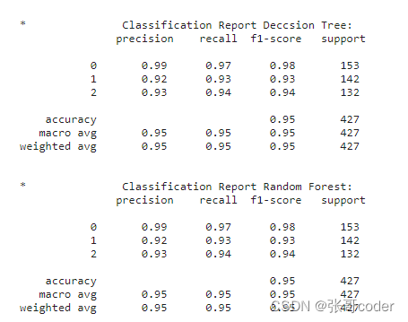
### Decision Tree Regressor

Classifier_dt = tree.DecisionTreeClassifier().fit(x_train, np.argmax(y_train,axis=1))
pred_dt = Classifier_dt.predict(x_test)
print ('\n*\t\tClassification Report Deccsion Tree:\n', classification_report(np.argmax(y_test,axis=1), pred_dt))
confusion_matrix_graph = confusion_matrix(np.argmax(y_test,axis=1), pred_dt)
### Random Forest

Classifier_forest = RandomForestClassifier(n_estimators = 50, random_state = 0).fit(x_train,np.argmax(y_train,axis=1))
pred_fr = Classifier_dt.predict(x_test)


print ('\n*\t\tClassification Report Random Forest:\n', classification_report(np.argmax(y_test,axis=1), pred_fr))
confusion_matrix_graph = confusion_matrix(np.argmax(y_test,axis=1), pred_fr)
fig, axes = plt.subplots(nrows=2, ncols=2, figsize=(15,10))
classifiers = [GaussianNB(),svm.SVC(kernel='linear'),
               linear_model.LogisticRegression(solver = 'liblinear', C = 75),
               RandomForestClassifier(n_estimators = 50, random_state = 0)]
from sklearn.metrics import plot_confusion_matrix
for cls in classifiers:
    cls.fit(x_train,np.argmax(y_train,axis=1))
    
colors = [ 'YlOrBr', 'GnBu', 'Pastel2', 'PuRd']
for cls, ax,c in zip(classifiers, axes.flatten(),colors):
    plot_confusion_matrix(cls, 
                          x_test, 
                          np.argmax(y_test,axis=1), 
                          ax=ax, 
                          cmap=c,
                         display_labels= names1)
    ax.title.set_text(type(cls).__name__)
plt.tight_layout()  
plt.show()

 

#Classification Report of Lstm model
print('\n*\t\tClassification Report OF Brain Waves LSTM:\n', classification_report(np.argmax(y_test,axis=1), np.argmax(lstmmodel.predict(x_test),axis=1) ))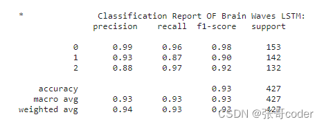

  

5 绘制模型训练loss和准确率

#Plotting Graph of Lstm model Training, Loss and Accuracy
plt.style.use("fivethirtyeight")
plt.figure(figsize = (20,6))
plt.subplot(1, 2, 1)
plt.plot(history.history['loss'])
plt.plot(history.history['val_loss'])
plt.title("Model Loss",fontsize=20)
plt.ylabel('Loss')
plt.xlabel('Epochs')
plt.legend(['train loss', 'validation loss'], loc ='best')

plt.subplot(1, 2, 2)
plt.plot(history.history['accuracy'])
plt.plot(history.history['val_accuracy'])
plt.title("Model Accuracy",fontsize=20)
plt.ylabel('Accuracy')
plt.xlabel('Epochs')
plt.legend(['training accuracy', 'validation accuracy'], loc ='best')
plt.show()

6 数据集下载

信号处理-基于EEG脑电信号的深度学习情绪分类 使用数据