TensorFlow 实现Linear Regression

下面使用TensorFlow实现线性回归，具体过程在代码中很详细。

# encoding:utf-8
import tensorflow as tf
import numpy as np
import matplotlib.pyplot as plt

# 定义参数，分别是学习率，迭代次数，还有一个是定义每50次迭代打印一些内容
learning_rate = 0.01
train_epochs = 1000
display_step = 50

# 定义一些训练数据
train_X = np.asarray([3.3, 4.4, 5.5, 6.71, 6.93, 4.168, 9.779, 6.182, 7.59, 2.167,
                      7.042, 10.791, 5.313, 7.997, 5.654, 9.27, 3.1])

train_Y = np.asarray([1.7, 2.76, 2.09, 3.19, 1.694, 1.573, 3.366, 2.596, 2.53, 1.221,
                      2.827, 3.465, 1.65, 2.904, 2.42, 2.94, 1.3])
n_samples = train_X.shape[0]


X = tf.placeholder(dtype='float')
Y = tf.placeholder(dtype='float')

# 定义两个需要求出的w和b变量
W = tf.Variable(np.random.randn(), name='weight')
b = tf.Variable(np.random.randn(), name='bias')

# 预测值
pre = tf.add(tf.mul(W, X), b)

# 定义代价损失和优化方法
cost = tf.reduce_sum(tf.pow(Y - pre, 2)) / (2 * n_samples)
optimizer = tf.train.GradientDescentOptimizer(learning_rate=0.01).minimize(cost)

# 以上整个图就定义好了

init = tf.initialize_all_variables()

# launch the graph
with tf.Session() as sess:
    sess.run(init)
    for epoch in range(train_epochs):
        for (x, y) in zip(train_X, train_Y):
            sess.run(optimizer, feed_dict={X: x, Y: y})
        # 每轮打印一些内容
        if (epoch + 1) % display_step == 0:
            c = sess.run(cost, feed_dict={X: train_X, Y: train_Y})
            print 'Epochs:', '%04d' % (epoch + 1), 'cost=', '{:.9f}'.format(c), 'W=', sess.run(W), 'b=', sess.run(b)
    print 'optimizer finished'
    training_cost = sess.run(cost, feed_dict={X: train_X, Y: train_Y})
    print "Training cost=", training_cost, "W=", sess.run(W), "b=", sess.run(b), '\n'
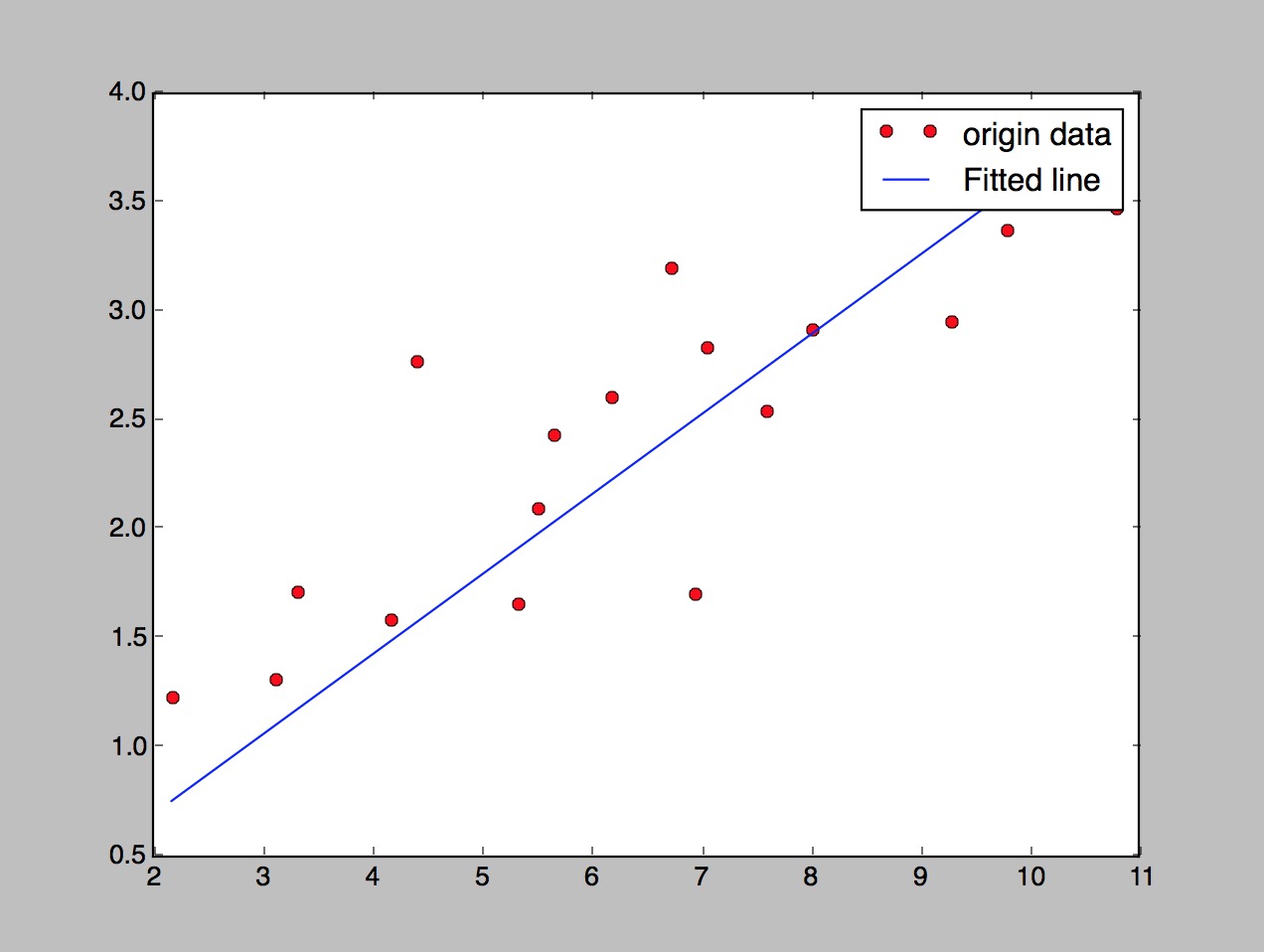
    # 画图
    plt.plot(train_X, train_Y, 'ro', label='origin data')
    plt.plot(train_X, sess.run(W) * train_X + sess.run(b), label='Fitted line')
    plt.legend()
    plt.show()

最后得到的w和b

optimizer finished
Training cost= 0.120649 W= 0.366514 b= -0.0396475 

最后的画图结果