【Python】Section 3: 模型选择和交叉验证 Model Selection and Cross-Validation from HarvardX_from train-test to cross-validation: advancing you-CSDN博客

本文链接：https://blog.csdn.net/Yqalu/article/details/138293205

1. Model Selection

1.1 Evaluation: Training Error

Just because we find a model that minimizes the squared error doesn't mean that it’s a good model. We should also investigate the $R^2$ as well. Consider these four models:

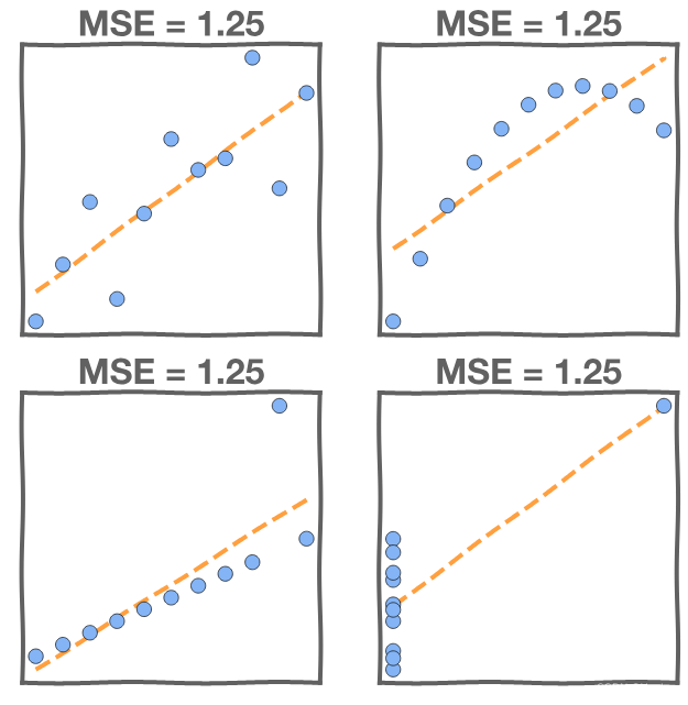
All four have the same MSE, but the fits to the data look very different. If MSE were our only criterion we would have to consider all models equally good. Let's add another criterion to our model selection to help us pick the right one.

1.2 Evaluation: Test Error

Definition: Generalization

The ability of a model to do well on new data is called generalization.

The goal of model selection is to choose the model that generalizes the best. To test if our model's performance generalizes to previously unseen examples we need to evaluate it on a separate set of data that the model did not train on. We call this the test data. Here's an example where our model fits the training set well but doesn't fit the test set. This is because the training data contains a strange point – an outlier – which confuses the model.

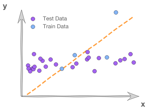
In general, we evaluate the model on both train and test data, because models that do well on training data may do poorly on new data. The training MSE here is 2.0, while the test MSE is 12.3. Evaluating the model on the test data makes it clear that the model doesn't work well for the full data set.

When a model is strongly influenced by aspects of its particular training data that do not generalize to new data we call this overfitting.

1.3 Model Selection

Model selection is the application of a principled method to determine the complexity of the model. This could be choosing a subset of predictors, choosing the degree of the polynomial model, etc.

A strong motivation for performing model selection is to avoid overfitting, which we saw can happen when:

there are too many predictors
the feature space has high dimensionality
the polynomial degree is too high
too many interaction terms are considered
the coefficients values are too extreme (we have not seen this yet)

Train-Test Split

So far, we have been using the train split to train a model and the test split to evaluate the model performance.

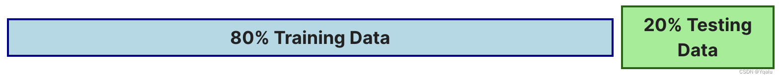
However, we can improve our methods by splitting the data again.

Train-Validation Split

As before, we use the train split to train a model and the test split to evaluate the final model's performance. But now we'll introduce a new sub-set, called validation, and use this to select the model.

1.4 Selection Approach

There are several approaches to model selection:

Exhaustive search (below)
Greedy algorithms (below)
Fine tuning hyper-parameters (later)
Regularization (later)

Exhaustive Search

Could we simply evaluate models trained on all possible combinations of predictors and select the best?

How many potential models are there when we have $J$ predictors and consider only linear terms?

For example, consider 3 predictors $X_1,X_2,X_3$ :

$\left.\begin{matrix} -\ Models\ with\ 0\ predictor:\\ M_0: bias\ only\\ -\ Models\ with\ 1\ predictor:\\ M_1:X_1\\ M_2:X_2\\ M_3:X_3\\ -\ Models\ with\ 2\ predictors:\\ M_4:\begin{Bmatrix} {X_1,X_3} \end{Bmatrix}\\ M_5:\begin{Bmatrix} {X_2,X_3} \end{Bmatrix}\\ M_6:\begin{Bmatrix} {X_3,X_1} \end{Bmatrix}\\ -\ Models\ with\ 3\ predictors:\\ M_7:\begin{Bmatrix} {X_1,X_2,X_3} \end{Bmatrix} \end{matrix}\right\}2^J\ models$

If we were able to evaluate all $2^J$ models we could be sure that we've selected the best among these candidates. However, this quickly becomes intractable as the number of predictors grows.

Greedy Algorithms

With a greedy algorithm we give up on trying to find the best possible model as this is not practical. Instead, we content ourselves with finding a locally optimal solution.

Stepwise Variable Selection and Validation

We then need to define a process for searching and selecting a (locally) optimal sub-set of predictors, including choosing the degree for polynomial models. One approach is stepwise variable selection and validation.

Here we iteratively building an optimal subset of predictors by optimizing a fixed model evaluation metric each time on a validation set. The algorithm is "greedy" in the sense that we are only concerned with optimization at the current iteration. There is a forward and a backward version of stepwise variable selection.

Stepwise Variable Selection: Forward Method

In forward selection, we find an 'optimal' set of predictors by iterative adding to our set.

Starting with the empty set $P_0$ , construct the null model, $M_0$ .
For :
1. Let $M_{k-1}$ be the model constructed from the best set of $k-1$ predictors, $P_{k-1}$ .
2. Select the predictor $X_{nk}$ , not in $P_{k-1}$ , so that the model constructed from $P_k=X_{nk}\bigcup P_{k-1}$ optimizes a fixed metric (this can be $p$ -value, F-stat, validation MSE, $R^2$ , or AIC/BIC on training set).
3. Let $M_k$ denote the model constructed from the optimal $P_k$ .
Select the model $M$ amongst $M_0,M_1,...,M_J$ that optimizes a fixed metric (this can be validation MSE, $R^2$ , or AIC/BIC on training set).

The computational complexity of stepwise variable selection computation is $O(J^2)<<2^J$ for large $J$ .

Fine tuning hyper-parameters

We can recast the problem of model selection as a problem of choosing hyper-parameters.

Definition: Hyper-Parameter

A hyper-parameter is a parameter of the model that is not itself learned from the data.

For example, polynomial regression requires choosing a degree – this can be thought of as model selection – and so we select a model by choosing a value for the hyper-parameter. This process of choosing a hyper-parameter value is called tuning.

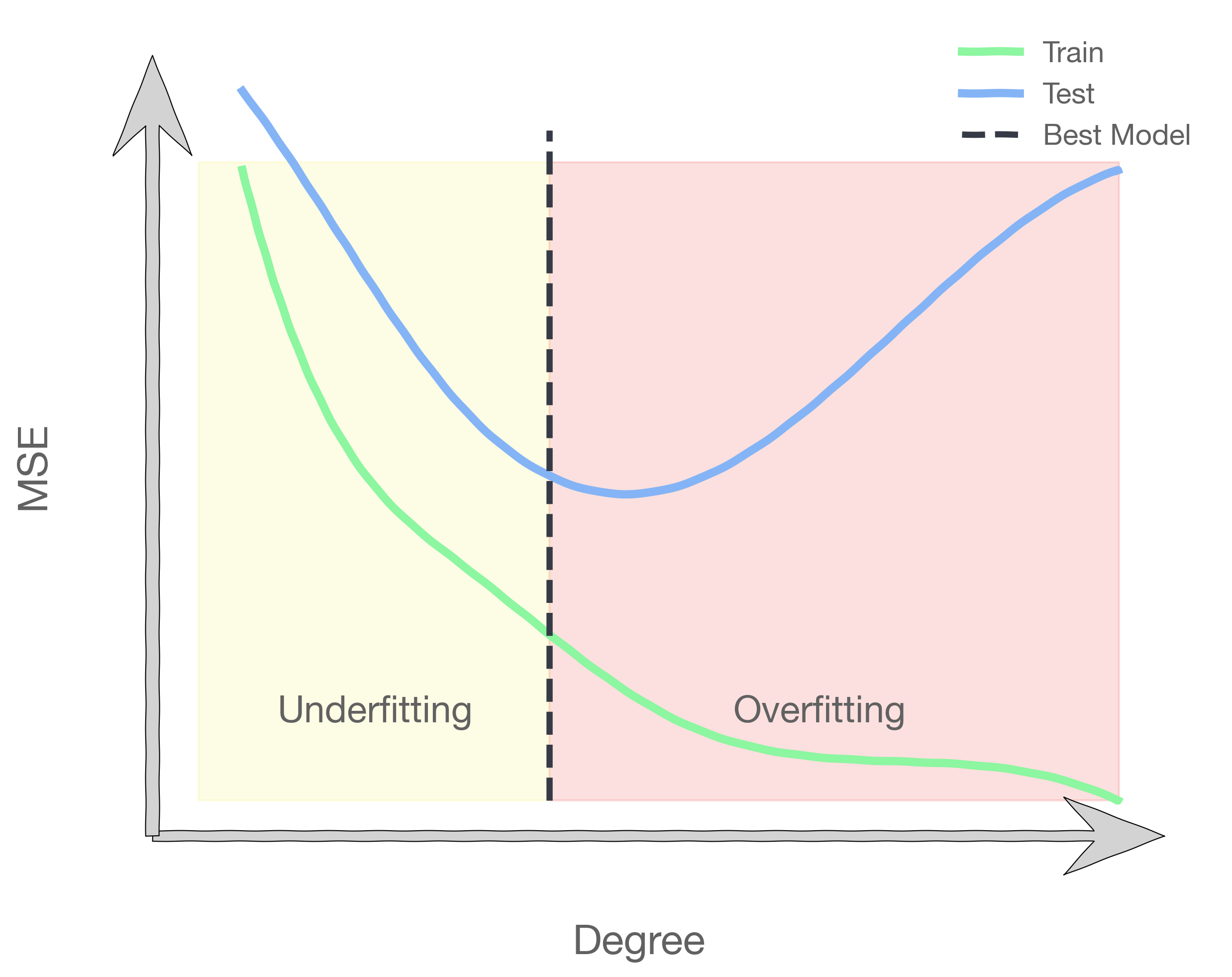
There are some hyper-parameters that we've seen before! For example, here are three models resulting from different choices of the polynomial degree fit on the same data. The degree of the polynomial is the hyper-parameter.

We observe that when the degree is too low the model will have high train and validation error. As the degree increases up to a point we see both errors decrease. But eventually the model will start to do worse on the validation data even as the training error continues to drop.

1.5 Evaluation: Model Interpretation

In addition to evaluating a model using a metric like MSE, we can also try to interpret the model and make to sure that what the model tells us makes sense.
For linear models we can interpret the parameters which are the $\beta$ 's.
Consider these two models, which you've seen before:

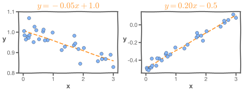
For the model on the left, the MSE of this model is very small. But the slope is -0.05. That means the larger the budget the less the sales. This isn't very likely. For the model on the right, the MSE is very small, but the intercept is -0.5 which means that for very small budget we will have negative sales which is not possible.

When we encounter nonsensical interpretations like these we should reinspect our modeling methodology and the data being used.

2. Cross-Validation

2.1 Motivation

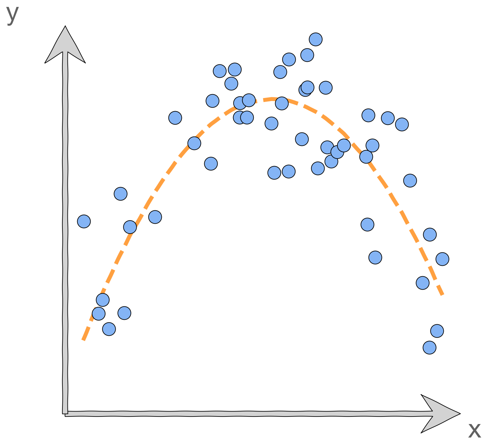
We've seen in the exercise a case where selecting a model's polynomial degree using validation loss gave us very poor results. The plot below shows another example of this.

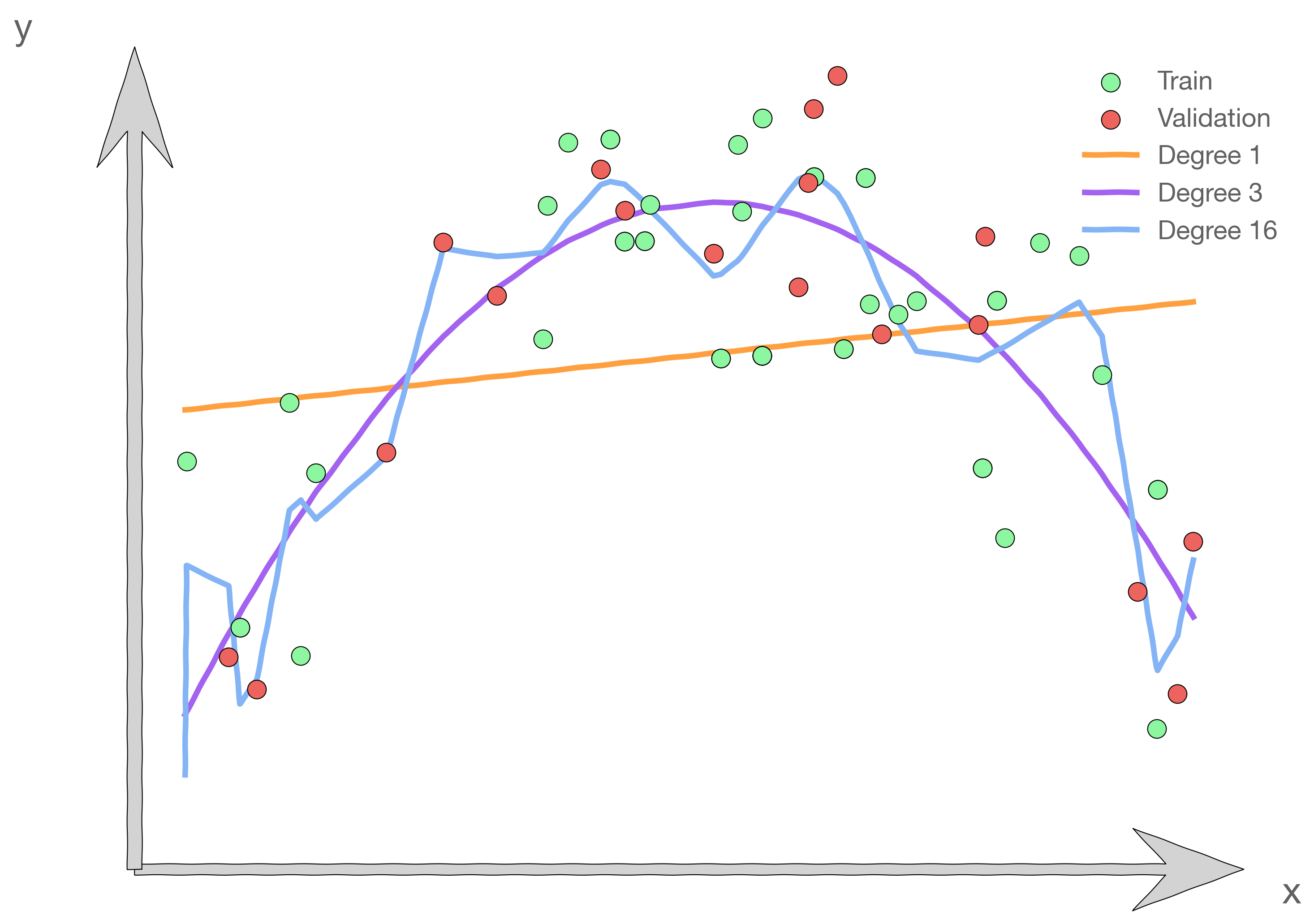
It is obvious that, out of the choices shown, a degree of 3 is the desired model. But the validation set by chance favors the linear model.

One solution to the problems raised by using a single validation set is to evaluate each model on multiple validation sets and average the validation performance. For example, one can randomly split the training set into training and validation multiple times but randomly creating these sets can create the scenario where important features of the data never appear in our random draws.

2.2 Cross-Validation

Recall that we use the train split of the data to train a model, the validation split to select the model, and the test split to evaluate the model performance. In the beginning, we always separated a portion of the data from the main dataset which we never touched until the very end. This is the test set we use to evaluate the performance of the final model.

We break down...

into...

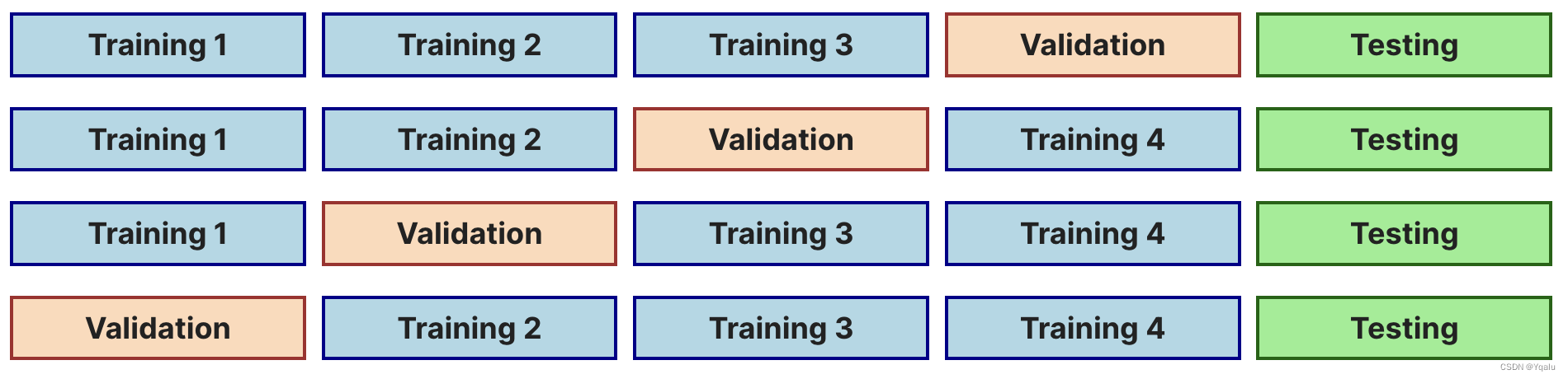
In cross validation, the train data is split into $k$ buckets or 'folds'. Then, iteratively, a new fold is used for validation and the remaining for training. This is repeated until all folds have been used as a validation set.

Validation Score

The validation score for cross validation is the average score across all $k$ validation folds:

$MSE^{val}=\frac{1}{k}\sum_{i=1}^{k}MSE_i^{val}$

Choosing number of folds

This is a choice we make (another hyper-parameter!), and it depends on the size of your data. We want every validation fold to have more than 50 or so data points and we want the spread of the validation MSE folds not to be too large. Five folds is a typical number we use.

When to use cross-validation

We may choose to use a single validation set rather than cross-validation if training takes too long as in the case of a very complex model like a deep neural network or when the dataset is large. Generally, the larger your dataset, the less sensitive your model selection process will be to your choice of validation set.