卷积核、池化层输出尺寸计算公式，VGG16神经网络结构图及各层推导及PyTorch实现代码

卷积层

  使用卷积处理图像，输出的图像的尺寸为：

$W_{out}=\frac{W_{in}-W_{filter}+2P}{S}+1$

$H_{out}=\frac{H_{in}-H_{filter}+2P}{S}+1$

  公式中$W_{filter}$和$H_{filter}$分别表示卷积核（filter）的宽和高。$P$（即padding）为在图像边缘填充的边界像素层数。$S$为步长（Stride）。

  图像在输入卷积层之前，有两种边界像素填充方式：

1. Same：在输入的图像最外层加上指定层数的像素值全为0的边界，这是为了让图像的全部像素都能被卷积核捕捉到；
2. Valid：不对输入的图像进行填充，直接对其进行卷积，这种方式的缺点就是可能导致一些像素不能被卷积核捕捉。

池化层

  池化层可以对原始数据进行压缩，减少模型的计算参数，提升运算效率。常用的池化层为：平均池化层和最大池化层。池化层处理的数据一般是经过卷积层处理后生层的特征图。

  经过池化层处理的图像，输出的图像的尺寸为：

$W_{out}=\frac{W_{in}-W_{filter}}{S}+1$

$H_{out}=\frac{H_{in}-H_{filter}}{S}+1$

  公式中$W_{filter}$和$H_{filter}$分别表示卷积核（filter）的宽和高。$W_{in}$、$H_{in}$和$W_{out}$、$H_{out}$分别代表输入、输出的特在图的宽和高。$S$为步长（Stride）。输入的特征图深度和卷积核深度一致。

VGGNet模型分析

  VGGNet是牛津大学计算机视觉组合和Google DeepMind公司研究员共同开发的深度卷积神经网络。是一个经典的神经网络。下面对其结构进行分析。这里对VGG16D进行分析。
  VGG16论文中给出的配置：

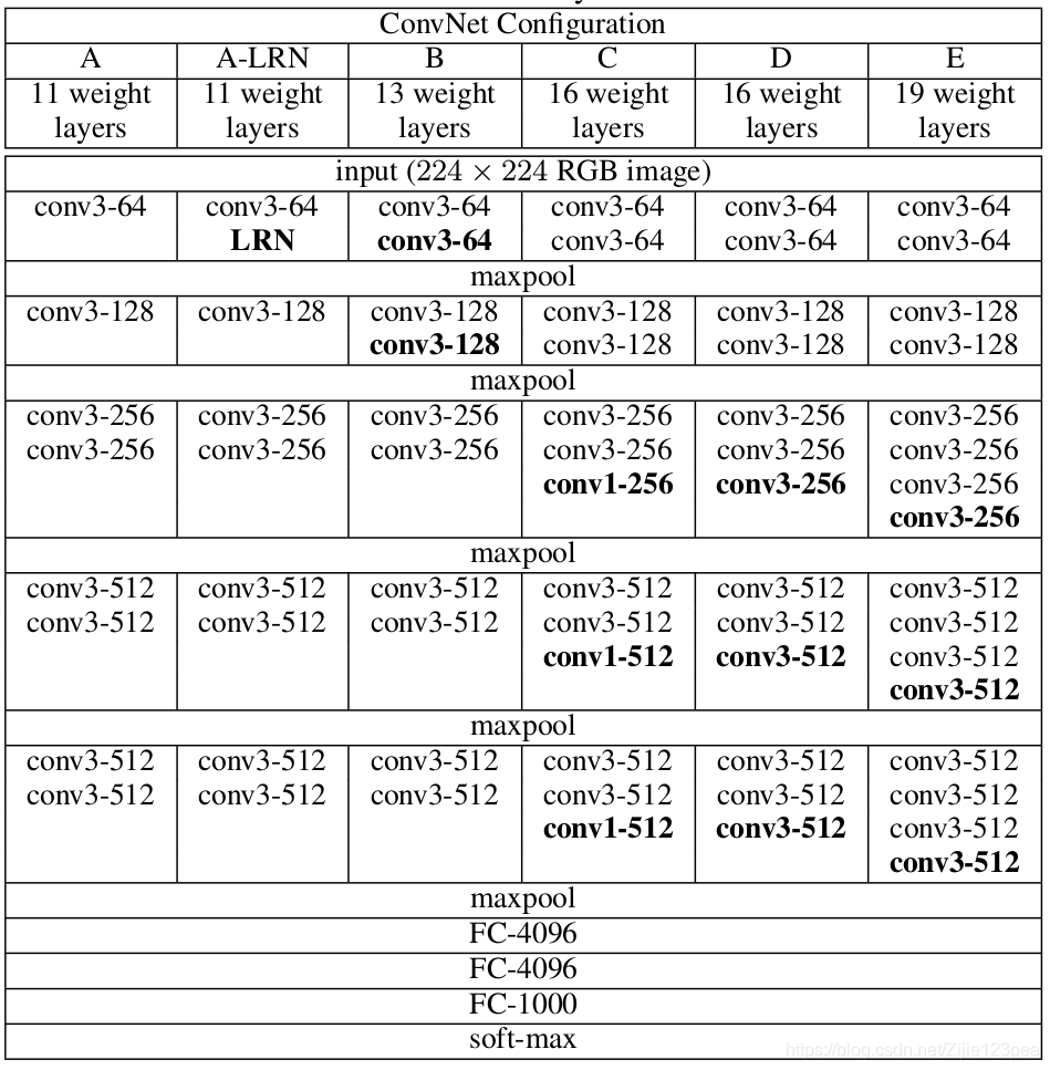
  特点：VGG16D卷积核滑动窗口尺寸统一为$3\times 3$（即感受野尺寸receptive field size为3），步长统一为1，有16层的VGG16模型和19层的VGG19模型两种类型。相对于AlexNet一共八层的结构，增加了层数。增加层数和更小的卷积核能有效提升模型的性能。

  分析：

（1）Input层：VGG16的卷积神经网络默认输入数据必须是$224\times 224\times 3$的图像，即高和宽224像素，色彩通道RGB3个，和AlexNet的要求是一致的。

（2）Conv1_1：卷积核维度为$3\times 3\times 3$，步长1，Padding为1。根据卷积核计算公式：

$W_{out}=\frac{W_{in}-W_{filter}+2P}{S}+1=\frac{224-3+2\times 1}{1}+1=224$

$H_{out}=\frac{H_{in}-H_{filter}+2P}{S}+1=\frac{224-3+2\times 1}{1}+1=224$

即输出的特征图高和宽都为224，该卷积层描述为：Conv1:64x224x224，即输出的特在图除了尺寸$224\times 224$外，还要深度为64，所以要进行64次卷积，最后输出的特征图维度为：$224\times 224\times 64$。

（3）Conv1_2：卷积核维度为$3\times 3\times 64$（卷积核的深度要与上层输出且输入本层的深度一致），步长1，Padding为1。根据卷积核计算公式：

$W_{out}=\frac{W_{in}-W_{filter}+2P}{S}+1=\frac{224-3+2\times 1}{1}+1=224$

$H_{out}=\frac{H_{in}-H_{filter}+2P}{S}+1=\frac{224-3+2\times 1}{1}+1=224$

由于输入特征图是上层的输出，所以Conv1_2的输入图片尺寸$224\times 224$，输出也是$224\times 224$。深度（即通道数）也是64，也是要进行64次卷积操作，最后输出的特征图维度为：$224\times 224\times 64$。
（4）Maxpool1：VGG16的所有池化层均为最大池化层，滑动窗口大小均为$2\times 2$，步长也均为2。
本池化层滑窗维度$2\times 2\times 64$（滑窗的深度要与上层输出且输入本层的深度一致）。由池化层计算公式得：

$W_{out}=\frac{W_{in}-W_{filter}}{S}+1=\frac{224-2}{2}+1=112$

$H_{out}=\frac{H_{in}-H_{filter}}{S}+1=\frac{224-2}{2}+1=112$

经过最大池化层后深度不变，所以，输出的特征图维度为$112\times 112\times 64$。

（5）Conv2_1：卷积核维度为$3\times 3\times 64$，步长1，Padding为1。根据卷积核计算公式：

$W_{out}=\frac{W_{in}-W_{filter}+2P}{S}+1=\frac{112-3+2\times 1}{1}+1=112$

$H_{out}=\frac{H_{in}-H_{filter}+2P}{S}+1=\frac{112-3+2\times 1}{1}+1=112$

由上面的表可知VGG16D在第三、第四个卷积层输出的通道数都为128，所以需要进行128次卷积操作，本层输出特征图维度$112\times 112\times 128$。

（6）Con2_2：卷积核维度为$3\times 3\times 128$，步长1，Padding为1。根据卷积核计算公式：

$W_{out}=\frac{W_{in}-W_{filter}+2P}{S}+1=\frac{112-3+2\times 1}{1}+1=112$

$H_{out}=\frac{H_{in}-H_{filter}+2P}{S}+1=\frac{112-3+2\times 1}{1}+1=112$

本层输出特征图维度$112\times 112\times 128$。

（7）Maxpool2：本池化层滑窗维度$2\times 2\times 128$，步长为2。由池化层计算公式得：

$W_{out}=\frac{W_{in}-W_{filter}}{S}+1=\frac{112-2}{2}+1=56$

$H_{out}=\frac{H_{in}-H_{filter}}{S}+1=\frac{112-2}{2}+1=56$

经过最大池化层后深度不变，所以，输出的特征图维度为$56\times 56\times 128$。

（8）Conv3_1:256x56x56：卷积核维度为$3\times 3\times 128$，步长1，Padding为1。根据卷积核计算公式：

$W_{out}=\frac{W_{in}-W_{filter}+2P}{S}+1=\frac{56-3+2\times 1}{1}+1=56$

$H_{out}=\frac{H_{in}-H_{filter}+2P}{S}+1=\frac{56-3+2\times 1}{1}+1=56$

表中参数可知，Conv3_1、Conv3_2和Conv3_3深度都是256,所以本层卷积256次，本层输出特征图维度$56\times 56\times 256$。
（9）Conv3_2:256x56x56：卷积核维度为$3\times 3\times 256$，步长1，Padding为1。根据卷积核计算公式：

$W_{out}=\frac{W_{in}-W_{filter}+2P}{S}+1=\frac{56-3+2\times 1}{1}+1=56$

$H_{out}=\frac{H_{in}-H_{filter}+2P}{S}+1=\frac{56-3+2\times 1}{1}+1=56$

表中参数可知，Conv3_1、Conv3_2和Conv3_3深度都是256,所以本层卷积256次，本层输出特征图维度$56\times 56\times 256$。
（10）Conv3_3:256x56x56：卷积核维度为$3\times 3\times 256$，步长1，Padding为1。根据卷积核计算公式：

$W_{out}=\frac{W_{in}-W_{filter}+2P}{S}+1=\frac{56-3+2\times 1}{1}+1=56$

$H_{out}=\frac{H_{in}-H_{filter}+2P}{S}+1=\frac{56-3+2\times 1}{1}+1=56$

表中参数可知，Conv3_1、Conv3_2和Conv3_3深度都是256,所以本层卷积256次，本层输出特征图维度$56\times 56\times 256$。
（11）Maxpool3:256x28x28：本池化层滑窗维度$2\times 2\times 256$，步长为2。由池化层计算公式得：

$W_{out}=\frac{W_{in}-W_{filter}}{S}+1=\frac{56-2}{2}+1=28$

$H_{out}=\frac{H_{in}-H_{filter}}{S}+1=\frac{56-2}{2}+1=28$

经过最大池化层后深度不变，所以，输出的特征图维度为$28\times 28\times 256$。
(12)Conv4_1:512x28x28：卷积核维度为$3\times 3\times 256$，步长1，Padding为1。根据卷积核计算公式：

$W_{out}=\frac{W_{in}-W_{filter}+2P}{S}+1=\frac{28-3+2\times 1}{1}+1=28$

$H_{out}=\frac{H_{in}-H_{filter}+2P}{S}+1=\frac{28-3+2\times 1}{1}+1=28$

表中参数可知，Conv4_1、Conv4_2和Conv4_3深度都是512,所以本层卷积512次，本层输出特征图维度$28\times 28\times 512$。
（13）Conv4_2:512x28x28：卷积核维度为$3\times 3\times 256$，步长1，Padding为1。根据卷积核计算公式：

$W_{out}=\frac{W_{in}-W_{filter}+2P}{S}+1=\frac{28-3+2\times 1}{1}+1=28$

$H_{out}=\frac{H_{in}-H_{filter}+2P}{S}+1=\frac{28-3+2\times 1}{1}+1=28$

表中参数可知，Conv4_1、Conv4_2和Conv4_3深度都是512,所以本层卷积512次，本层输出特征图维度$28\times 28\times 512$。
（14）Conv4_3:512x28x28：卷积核维度为$3\times 3\times 256$，步长1，Padding为1。根据卷积核计算公式：

$W_{out}=\frac{W_{in}-W_{filter}+2P}{S}+1=\frac{28-3+2\times 1}{1}+1=28$

$H_{out}=\frac{H_{in}-H_{filter}+2P}{S}+1=\frac{28-3+2\times 1}{1}+1=28$

表中参数可知，Conv4_1、Conv4_2和Conv4_3深度都是512,所以本层卷积512次，本层输出特征图维度$28\times 28\times 512$。
（15）Maxpool4:512x14x14：本池化层滑窗维度$2\times 2\times 512$，步长为2。由池化层计算公式得：

$W_{out}=\frac{W_{in}-W_{filter}}{S}+1=\frac{28-2}{2}+1=14$

$H_{out}=\frac{H_{in}-H_{filter}}{S}+1=\frac{28-2}{2}+1=14$

经过最大池化层后深度不变，所以，输出的特征图维度为$14\times 14\times 512$。
（16）Conv5_1:512x14x14：卷积核维度为$3\times 3\times 512$，步长1，Padding为1。根据卷积核计算公式：

$W_{out}=\frac{W_{in}-W_{filter}+2P}{S}+1=\frac{14-3+2\times 1}{1}+1=14$

$H_{out}=\frac{H_{in}-H_{filter}+2P}{S}+1=\frac{14-3+2\times 1}{1}+1=14$

表中参数可知，Conv5_1、Conv5_2和Conv5_3深度都是512,所以本层卷积512次，本层输出特征图维度$14\times 14\times 512$。
（17）Conv5_2:512x14x14：卷积核维度为$3\times 3\times 512$，步长1，Padding为1。根据卷积核计算公式：

$W_{out}=\frac{W_{in}-W_{filter}+2P}{S}+1=\frac{14-3+2\times 1}{1}+1=14$

$H_{out}=\frac{H_{in}-H_{filter}+2P}{S}+1=\frac{14-3+2\times 1}{1}+1=14$

表中参数可知，Conv5_1、Conv5_2和Conv5_3深度都是512,所以本层卷积512次，本层输出特征图维度$14\times 14\times 512$。
（18）Conv5_3:512x14x14：卷积核维度为$3\times 3\times 512$，步长1，Padding为1。根据卷积核计算公式：

$W_{out}=\frac{W_{in}-W_{filter}+2P}{S}+1=\frac{14-3+2\times 1}{1}+1=14$

$H_{out}=\frac{H_{in}-H_{filter}+2P}{S}+1=\frac{14-3+2\times 1}{1}+1=14$

表中参数可知，Conv5_1、Conv5_2和Conv5_3深度都是512,所以本层卷积512次，本层输出特征图维度$14\times 14\times 512$。
（19）Maxpool5:512x7x7：本池化层滑窗维度$2\times 2\times 512$，步长为2。由池化层计算公式得：

$W_{out}=\frac{W_{in}-W_{filter}}{S}+1=\frac{14-2}{2}+1=7$

$H_{out}=\frac{H_{in}-H_{filter}}{S}+1=\frac{14-2}{2}+1=7$

经过最大池化层后深度不变，所以，输出的特征图维度为$7\times 7\times 512$。
（20）FC13:4096：全连接层，输入的特征图维度为$7\times 7\times 512$，和AlexNet一样都要先对该输入的特征图扁平化，即$7\times 7\times 512=1\times 25088$，把特征图变成$1\times 25088$的数据。由表可知，输出数据的深度为$1\times 4096$，所以需要一个$25088\times 4096$的参数矩阵完成输入数据和输出数据的全连接，实质为线性方程组，即：

$\left[\begin{array}{cccc}{x}_1& x_2& \dots & x_{25088}\end{array}\right]\left[\begin{array}{cccc}{\theta }_{1-1}& {\theta }_{2-1}& \dots & {\theta }_{4096-1}\\ {\theta }_{1-2}& {\theta }_{2-2}& \dots & {\theta }_{4096-2}\\ ⋮& ⋮& \ddots & ⋮\\ {\theta }_{1-25088}& {\theta }_{2-25088}& \dots & {\theta }_{4096-25088}\end{array}\right]=\left[\begin{array}{cccc}{\sum }_{i=1}^{25088}{x}_i{\theta }_{1-i}& {\sum }_{i=1}^{25088}{x}_i{\theta }_{2-i}& \dots & {\sum }_{i=1}^{25088}{x}_i{\theta }_{4096-i}\end{array}\right]=FC4096$

其中，例如，$a{x}_1$表示第一个变量，${\theta }_{2-1}$表示第二组数据（每组数据就是一个深度）的第一个参数。$FC4096$就是本全连接层输出的结果，维度$1\times 4096$。
（21）FC14:4096：输入数据的维度：$1\times 4096$，输出数据维度也要求是$1\times 4096$，所以，连接矩阵维度为$4096\times 4096$，矩阵乘法如下：

$\left[\begin{array}{cccc}F{C}_1& F{C}_2& \dots & F{C}_{4096}\end{array}\right]\left[\begin{array}{cccc}{\alpha }_{1-1}& {\alpha }_{2-1}& \dots & {\alpha }_{4096-1}\\ {\alpha }_{1-2}& {\alpha }_{2-2}& \dots & {\alpha }_{4096-2}\\ ⋮& ⋮& \ddots & ⋮\\ {\alpha }_{1-4096}& {\alpha }_{2-4096}& \dots & {\alpha }_{4096-4096}\end{array}\right]=\left[\begin{array}{cccc}{\sum }_{i=1}^{4096}F{C}_i{\alpha }_{1-i}& {\sum }_{i=1}^{4096}F{C}_i{\alpha }_{2-i}& \dots & {\sum }_{i=1}^{4096}F{C}_i{\alpha }_{4096-i}\end{array}\right]=FC4096_2$

$FC4096_2$就是本全连接层输出的结果，维度$1\times 4096$。
（22）FC15:1000：输入数据的维度：$1\times 4096$，输出数据维度要求是$1\times 1000$，所以，连接矩阵维度为$4096\times 1000$，矩阵乘法如下：

$\left[\begin{array}{cccc}F{C}_{2-1}& F{C}_{2-2}& \dots & F{C}_{2-4096}\end{array}\right]\left[\begin{array}{cccc}{\gamma }_{1-1}& {\gamma }_{2-1}& \dots & {\gamma }_{1000-1}\\ {\gamma }_{1-2}& {\gamma }_{2-2}& \dots & {\gamma }_{1000-2}\\ ⋮& ⋮& \ddots & ⋮\\ {\gamma }_{1-4096}& {\gamma }_{2-4096}& \dots & {\gamma }_{1000-4096}\end{array}\right]=\left[\begin{array}{cccc}{\sum }_{i=1}^{4096}F{C}_{2-i}{\gamma }_{1-i}& {\sum }_{i=1}^{4096}F{C}_{2-i}{\gamma }_{2-i}& \dots & {\sum }_{i=1}^{4096}F{C}_{2-i}{\gamma }_{4096-i}\end{array}\right]=FC4096_3$

$FC4096_3$就是本全连接层输出的结果，维度$1\times 1000$。

（23）Outpu:1000：输出层，实质是个Softmax层，将全连接层最后输出的维度为$1\times 1000$的数据传入Softmax函数中，就可以得到1000个预测值，这1000个预测值就是模型预测的输入图像所对应的每个类别的可能性。

PyTorch代码实现

  下面使用PyTorch来实现VGG16网络。
  使用的函数：

torch.nn.Conv2d()：

  用来搭建卷积神经网络的卷积层.
  例如上面的Conv1_1层，卷积核维度为$3\times 3\times 3$，步长1，Padding为1，输出的特征图深度为64，所以要进行64次卷积，最后输出的特征图维度为：$224\times 224\times 64$。
实现：

torch.nn.Conv2d(3, 64, kernel_size=3, stride=1, padding=1)   #第一个参数是本层输入通道数，第二个是本层输出通道数。

  Conv1_2层：卷积核维度为$3\times 3\times 64$（卷积核的深度要与上层输出且输入本层的深度一致），步长1，Padding为1。Conv1_2的输入图片尺寸$224\times 224$，输出也是$224\times 224$。深度（即通道数）也是64，也是要进行64次卷积操作，最后输出的特征图维度为：$224\times 224\times 64$。
实现：

torch.nn.Conv2d(64, 64, kernel_size=3, stride=1, padding=1)

torch.nn.ReLU()：

  ReLU层，每个卷积层后跟一个ReLU层。
实现：

torch.nn.ReLU()

torch.nn.MaxPool2d()

  用于实现神经网络中的最大池化层，输入的参数分别为池化窗口大小、池化窗口移动步长和Padding值。

  例如，第一个池化层：Maxpool1：VGG16的所有池化层均为最大池化层，滑动窗口大小均为$2\times 2$，步长也均为2。本池化层滑窗维度$2\times 2\times 64$（滑窗的深度要与上层输出且输入本层的深度一致）。经过最大池化层后深度不变，所以，输出的特征图维度为$112\times 112\times 64$。
实现（无padding，所以第三个参数缺省）：

torch.nn.MaxPool2d(kernel_size=2, stride=2)

torch.nn.Linear()

  全连接层用这个函数实现，实质是做$y=wx+b$的矩阵运算。
  例如：第一个全连接层FC13:4096：输入的特征图维度为$7\times 7\times 512$，它会先对该输入的特征图扁平化，即$7\times 7\times 512=1\times 25088$，把特征图变成$1\times 25088$的数据。由表可知，输出数据的深度为$1\times 4096$，所以需要一个$25088\times 4096$的参数矩阵完成输入数据和输出数据的全连接，实质为线性方程组，即：

$\left[\begin{array}{cccc}{x}_1& x_2& \dots & x_{25088}\end{array}\right]\left[\begin{array}{cccc}{\theta }_{1-1}& {\theta }_{2-1}& \dots & {\theta }_{4096-1}\\ {\theta }_{1-2}& {\theta }_{2-2}& \dots & {\theta }_{4096-2}\\ ⋮& ⋮& \ddots & ⋮\\ {\theta }_{1-25088}& {\theta }_{2-25088}& \dots & {\theta }_{4096-25088}\end{array}\right]=\left[\begin{array}{cccc}{\sum }_{i=1}^{25088}{x}_i{\theta }_{1-i}& {\sum }_{i=1}^{25088}{x}_i{\theta }_{2-i}& \dots & {\sum }_{i=1}^{25088}{x}_i{\theta }_{4096-i}\end{array}\right]=FC4096$

其中，例如，$a{x}_1$表示第一个变量，${\theta }_{2-1}$表示第二组数据（每组数据就是一个深度）的第一个参数。$FC4096$就是本全连接层输出的结果，维度$1\times 4096$。
实现：

torch.nn.Linear(in_features=7*7*512, out_features=4096)

  注意，第一个参数是输入的数据维度，第二个为输出数据维度，第三个参数为布尔值，缺省表示True，系统自动生成偏置项，如果False则表示无偏置项目。

torch.nn.Dropout()

  函数torch.nn.Dropout()用于防止神经网络过拟合，其原理是，在训练过程中，以一定几率将模型的部分参数变成0，以达到减少两层网络之间的连接的目的。
实现：

torch.nn.Dropout(p=0.5)   #以0.5的概率来归零神经元的参数

总体代码

import torch

class Models(torch.nn.Module):

    def __init__(self):
        super(Models, self).__init__()
        self.Conv = torch.nn.Sequential(
            torch.nn.Conv2d(3, 64, kernel_size=3, stride=1, padding=1),
            torch.nn.ReLU(),
            torch.nn.Conv2d(64, 64, kernel_size=3, stride=1, padding=1),
            torch.nn.ReLU(),
            torch.nn.MaxPool2d(kernel_size=2, stride=2),

            torch.nn.Conv2d(64, 128, kernel_size=3, stride=1, padding=1),
            torch.nn.ReLU(),
            torch.nn.Conv2d(128, 128, kernel_size=3, stride=1, padding=1),
            torch.nn.ReLU(),
            torch.nn.MaxPool2d(kernel_size=2, stride=2),

            torch.nn.Conv2d(128, 256, kernel_size=3, stride=1, padding=1),
            torch.nn.ReLU(),
            torch.nn.Conv2d(256, 256, kernel_size=3, stride=1, padding=1),
            torch.nn.ReLU(),
            torch.nn.Conv2d(256, 256, kernel_size=3, stride=1, padding=1),
            torch.nn.ReLU(),
            torch.nn.MaxPool2d(kernel_size=2, stride=2),

            torch.nn.Conv2d(256, 512, kernel_size=3, stride=1, padding=1),
            torch.nn.ReLU(),
            torch.nn.Conv2d(512, 512, kernel_size=3, stride=1, padding=1),
            torch.nn.ReLU(),
            torch.nn.Conv2d(512, 512, kernel_size=3, stride=1, padding=1),
            torch.nn.ReLU(),
            torch.nn.MaxPool2d(kernel_size=2, stride=2)
			
			torch.nn.Conv2d(512, 512, kernel_size=3, stride=1, padding=1),
            torch.nn.ReLU(),
            torch.nn.Conv2d(512, 512, kernel_size=3, stride=1, padding=1),
            torch.nn.ReLU(),
            torch.nn.Conv2d(512, 512, kernel_size=3, stride=1, padding=1),
            torch.nn.ReLU(),
            torch.nn.MaxPool2d(kernel_size=2, stride=2)

        )

        self.FC = torch.nn.Sequential(
            torch.nn.Linear(in_features=7*7*512, out_features=4096),
            torch.nn.ReLU(),
            torch.nn.Dropout(p=0.5),
            torch.nn.Linear(in_features=4096, out_features=4096),
            torch.nn.ReLU(),
            torch.nn.Dropout(p=0.5),
            torch.nn.Linear(in_features=4096, out_features=10)

        )

    def forward(self, x):
        x = self.Conv(x)
        x = x.view(-1, 7*7*512)
        x = self.FC(x)
        return x

model = Models()    #实例化Models类
print(model)     #打印输出模型结构