基于轻量级CNN的图像识别

轻量级算法

目前较流行的轻量级算法有很多，但是文章里主要用了MobileNetV2、ShuffleNetV2、SqueezeNet三种，但是对于千级的数据集还是需要很长的处理时间

• 目录

  轻量级算法

  前言

  一、数据集

  二、算法实现

  1.导包

  2.图像归一化

  3.加载模型

  4.训练模型

  5.算法对比

  总结

  ---

---

前言

对比了三种轻量级算法，有MobileNetV2、ShuffleNetV2、SqueezeNet，做岩石图片的三分类

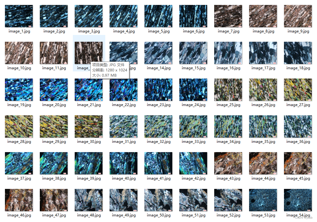
一、数据集

采用的是南京大学岩石薄片教学公开数据集，南京大学岩石薄片数据集，手动分成训练集和测试集，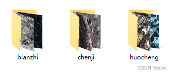

二、算法实现

1.导包

代码如下（示例）：

import torch
import torch.nn as nn
import torch.optim as optim
from torchvision import models, transforms
from torchvision.datasets import ImageFolder
from torch.utils.data import DataLoader
from sklearn.metrics import accuracy_score, recall_score, f1_score, precision_score
import csv
import datetime

2.图像归一化

代码如下（示例）：

# 数据预处理
transform = transforms.Compose([
    transforms.Resize(224),
    transforms.CenterCrop(224),
    transforms.ToTensor(),
    transforms.Normalize(mean=[0.485, 0.456, 0.406], std=[0.229, 0.224, 0.225])
])

# 加载数据集
train_dataset = ImageFolder('../202310/Stone-image/train', transform=transform)
test_dataset = ImageFolder('../202310/Stone-image/test', transform=transform)

train_loader = DataLoader(train_dataset, batch_size=32, shuffle=True)
test_loader = DataLoader(test_dataset, batch_size=32, shuffle=False)

3.加载模型

三种算法都是类似的，可以直接从pytorch官网上找到

# 初始化模型并设置输出类别数为3
model = models.shufflenet_v2_x1_0(num_classes=3)

# 定义损失函数和优化器
criterion = nn.CrossEntropyLoss()
optimizer = optim.Adam(model.parameters(), lr=0.0001)

4.训练模型

# 训练循环
num_epochs = 100

for epoch in range(num_epochs):
    running_loss = 0.0
    correct = 0
    total = 0

    for inputs, labels in train_loader:
        optimizer.zero_grad()

        outputs = model(inputs)
        loss = criterion(outputs, labels)
        loss.backward()
        optimizer.step()

        running_loss += loss.item() * inputs.size(0)
        _, predicted = torch.max(outputs.data, 1)
        total += labels.size(0)
        correct += (predicted == labels).sum().item()

    train_loss = running_loss / total
    train_accuracy = correct / total


    # 在测试集上评估模型
    with torch.no_grad():
        model.eval()
        test_correct = 0
        test_total = 0
        test_pred = []
        test_true = []

        for inputs, labels in test_loader:
            outputs = model(inputs)
            _, predicted = torch.max(outputs.data, 1)
            test_total += labels.size(0)
            test_correct += (predicted == labels).sum().item()


        test_accuracy = test_correct / test_total
        test_precision = precision_score(test_true, test_pred, average='weighted',zero_division=0)
        test_recall = recall_score(test_true, test_pred, average='weighted',zero_division=0)
        test_f1 = f1_score(test_true, test_pred, average='weighted',zero_division=0)



    print(f'Epoch [{epoch + 1}/{num_epochs}], Train Loss: {train_loss:.4f}, Train Accuracy: {train_accuracy:.4f}')
    print(f'Test Accuracy: {test_accuracy:.4f}, Test Precision: {test_precision:.4f}, Test Recall: {test_recall:.4f}, Test F1: {test_f1:.4f}')


# 输出最终测试集上的精确率、召回率和F1值
print(f"Final Test Results: Accuracy={test_accuracy:.4f}, Precision={test_precision:.4f}, Recall={test_recall:.4f}, F1 Score={test_f1:.4f}")
test_accuracy1.write(f"ShuffleNetV2 Final Test Results: Accuracy={test_accuracy:.4f}, Precision={test_precision:.4f}, Recall={test_recall:.4f}, F1 Score={test_f1:.4f}")

5.算法对比

plt.figure(figsize=(12, 6))


plt.subplot(3, 2, 1)
plt.plot(x, y1_loss, label='MobileNetV2')
plt.plot(x, y2_loss, label='ShuffleNetV2')
plt.plot(x, y3_loss, label='SqueezeNet')
plt.title('Train Loss Lines')
plt.legend()
plt.xlabel('x')
plt.ylabel('y')


plt.subplot(3, 2, 2)
plt.plot(x, y1_train_accuracy, label='MobileNetV2')
plt.plot(x, y2_train_accuracy, label='ShulleNetV2')
plt.plot(x, y3_train_accuracy, label='SqueezeNet')
plt.title('Train Accuracy Lines')
plt.xlabel('x')
plt.ylabel('y')

plt.subplot(3, 2, 3)
plt.plot(x, y1_accuracy, label='MobileNetV2')
plt.plot(x, y2_accuracy, label='ShulleNetV2')
plt.plot(x, y3_accuracy, label='SqueezeNet')
plt.title('Test Accuracy Lines')
plt.xlabel('x')
plt.ylabel('y')

plt.subplot(3, 2, 4)
plt.plot(x, y1_precision, label='MobileNetV2')
plt.plot(x, y2_precision, label='ShulleNetV2')
plt.plot(x, y3_precision, label='SqueezeNet')
plt.title('Test Precision Lines')
plt.xlabel('x')
plt.ylabel('y')

plt.subplot(3, 2, 5)
plt.plot(x, y1_recall, label='MobileNetV2')
plt.plot(x, y2_recall, label='ShulleNetV2')
plt.plot(x, y3_recall, label='SqueezeNet')
plt.title('Test Recall Lines')
plt.xlabel('x')
plt.ylabel('y')

plt.subplot(3, 2, 6)
plt.plot(x, y1_f1, label='MobileNetV2')
plt.plot(x, y2_f1, label='ShulleNetV2')
plt.plot(x, y3_f1, label='SqueezeNet')
plt.title('Test F1 Lines')
plt.xlabel('x')
plt.ylabel('y')



# 调整子图参数，使之填充整个图像区域
plt.tight_layout()

# 显示图形
plt.show()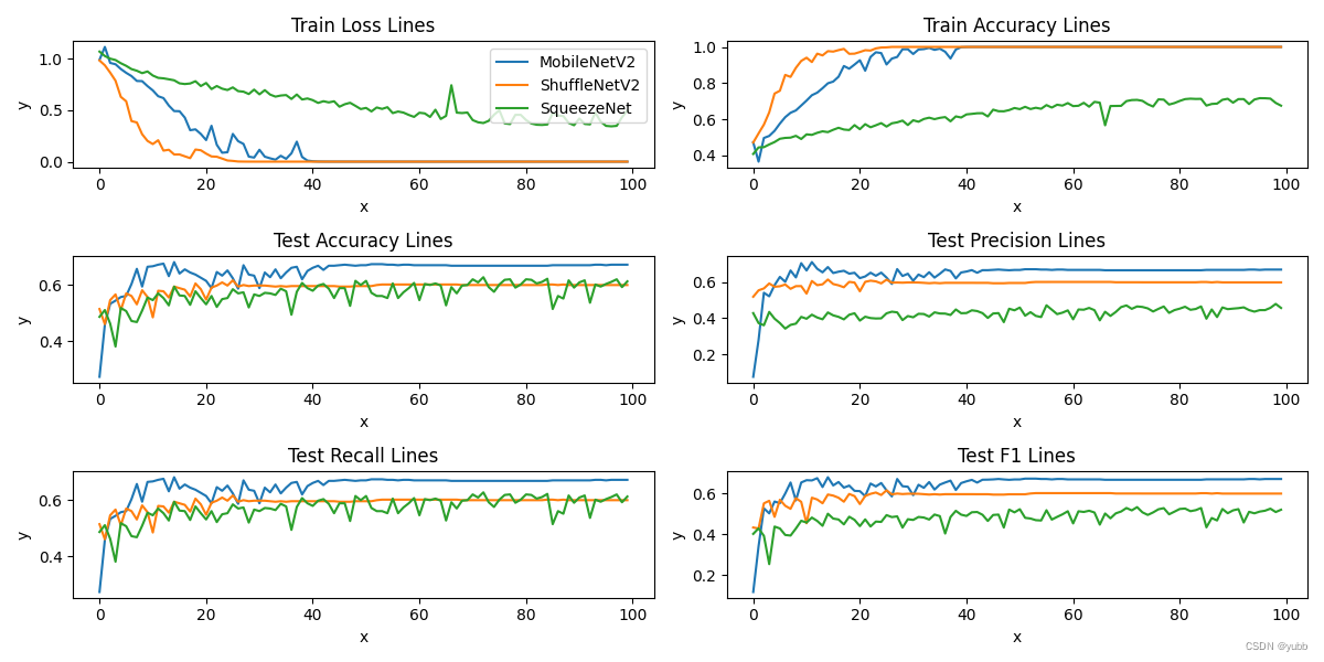

在训练集上ShuffleNet的收敛速度更快，在测试集上MobileNet的精度更高，各有千秋，ShuffleNet 是由于加入了通道混洗的模块所以在训练速度上更快。                                                                   

---

总结

整个流程就是如上，如果能结合两种算法的优点就更好了，做到模型融合。