from sklearn. model_selection import GridSearchCV
import time
from xgboost import XGBRegressor
from sklearn import preprocessing
from sklearn. metrics import mean_squared_error, r2_score
from sklearn. model_selection import train_test_split, KFold
import pandas as pd
import numpy as np
import matplotlib. pyplot as plt
from utils import *
from sklearn. model_selection import GridSearchCV
x_train, x_test, y_train, y_test= load_dataset( './datasets/xxxxxx.csv' )
def main ( ) :
start = time. clock( )
estimator = XGBRegressor( learning_rate= 0.05 , max_depth= 6 , n_estimators= 700 )
'''
参数空间
'''
learning_rate = [ 0.01 , 0.05 , 0.1 ]
n_estimators = [ 700 , 900 , 1100 , 1300 ]
max_depth = [ 6 , 10 , 15 , 20 ]
param_grid = dict (
learning_rate = learning_rate,
n_estimators = n_estimators,
max_depth= max_depth)
kflod= KFold( n_splits= 5 , shuffle= True )
print ( "Begin Train" )
grid_search = GridSearchCV( estimator, param_grid, scoring = 'neg_mean_squared_error' , n_jobs = - 1 , cv = kflod)
grid_result = grid_search. fit( x_train, y_train)
print ( "Best: %f using %s" % ( grid_result. best_score_, grid_search. best_params_) )
means = grid_result. cv_results_[ 'mean_test_score' ]
params = grid_result. cv_results_[ 'params' ]
for mean, param in zip ( means, params) :
print ( "%f with: %r" % ( mean, param) )
from sklearn. model_selection import RandomizedSearchCV
param_dist = {
'n_estimators' : range ( 1 , 1500 , 50 ) ,
'max_depth' : range ( 1 , 16 , 1 ) ,
'learning_rate' : np. linspace( 0.001 , 0.9 ) ,
}
model= XGBRegressor( )
grid = RandomizedSearchCV( model, param_dist, cv = 3 , scoring = 'neg_mean_squared_error' , n_iter= 100 , n_jobs = - 1 )
grid. fit( x_train, y_train)
best_estimator = grid. best_estimator_
print ( best_estimator)
print ( grid. best_score_)
from bayes_opt import BayesianOptimization
def xgb_cv ( max_depth, learning_rate, n_estimators) :
val = cross_val_score( estimator= XGBRegressor( max_depth= int ( max_depth) ,
learning_rate= learning_rate,
n_estimators= int ( n_estimators) ,
objective= 'reg:squarederror' ,
booster= 'gbtree' ,
seed= 0 ) , X= x_train, y= y_train, scoring= 'neg_mean_squared_error' , cv= 10 ) . mean( )
return val
xgb_bo = BayesianOptimization( xgb_cv, pbounds= { 'max_depth' : ( 1 , 16 ) ,
'learning_rate' : ( 0.001 , 0.9 ) ,
'n_estimators' : ( 1 , 1500 ) ,
} )
xgb_bo. maximize( n_iter= 100 , init_points= 10 )
print ( xgb_bo. max )
import optuna
def objective ( trial) :
max_depth = trial. suggest_int( 'max_depth' , 1 , 16 )
learning_rate = trial. suggest_uniform( 'learning_rate' , 0.001 , 0.9 )
n_estimators = trial. suggest_int( 'n_estimators' , 50 , 1500 , step= 50 )
estimator = XGBRegressor(
objective= 'reg:squarederror' ,
learning_rate = learning_rate,
n_estimators = n_estimators,
max_depth = max_depth,
seed = 0 )
estimator. fit( x_train, y_train)
val_pred = estimator. predict( x_test)
rmse = np. sqrt( mean_squared_error( y_test, val_pred) )
return rmse
study = optuna. create_study( sampler= optuna. samplers. TPESampler( ) , direction= 'minimize' )
start_time = time. time( )
study. optimize( objective, n_trials= 100 )
end_time = time. time( )
elapsed_mins, elapsed_secs = epoch_time( start_time, end_time)
print ( 'elapsed_secs:' , elapsed_secs)
print ( 'Best value:' , study. best_trial. value)
from hyperopt import fmin, hp, partial, Trials, tpe, rand
def cat_factory ( argsDict) :
estimator = XGBRegressor(
objective= 'reg:squarederror' ,
learning_rate= argsDict[ 'learning_rate' ] ,
n_estimators= int ( argsDict[ 'n_estimators' ] ) ,
max_depth= int ( argsDict[ 'max_depth' ] ) ,
seed= 0 )
estimator. fit( x_train, y_train)
val_pred = estimator. predict( x_test)
rmse = np. sqrt( mean_squared_error( y_test, val_pred) )
return rmse
algo = partial( tpe. suggest)
trials = Trials( )
start_time = time. time( )
best = fmin( cat_factory, space, algo= algo, max_evals= 100 , trials= trials)
end_time = time. time( )
elapsed_mins, elapsed_secs = epoch_time( start_time, end_time)
print ( 'elapsed_secs:' , elapsed_secs)
all_opts = [ ]
for one in trials:
str_re = str ( one)
argsDict = one[ 'misc' ] [ 'vals' ]
value = one[ 'result' ] [ 'loss' ]
learning_rate = argsDict[ "learning_rate" ] [ 0 ]
n_estimators = argsDict[ "n_estimators" ] [ 0 ]
max_depth = argsDict[ "max_depth" ] [ 0 ]
finish = [ value, learning_rate, n_estimators, max_depth]
all_opts. append( finish)
parameters = pd. DataFrame( all_opts, columns= [ 'value' , 'learning_rate' , 'n_estimators' , 'max_depth' ] )
best = parameters. loc[ abs ( parameters[ 'value' ] ) . idxmin( ) ]
print ( "best: {}" . format ( best) )
import torch
import torch. nn as nn
import numpy as np
from ray import tune
import pandas as pd
import matplotlib. pyplot as plt
from sklearn. model_selection import train_test_split
from sklearn. datasets import load_boston
def normalize ( x_data, mean, deviation) :
std = ( x_data - mean) / deviation
return std
def draw ( y1_axis, y2_axis) :
from sklearn. metrics import mean_squared_error, r2_score, mean_absolute_error
y1_axis= y1_axis. detach( ) . numpy( )
y2_axis = y2_axis. detach( ) . numpy( )
rmse= np. sqrt( mean_squared_error( y1_axis, y2_axis) )
mae= mean_absolute_error( y1_axis, y2_axis)
r2= r2_score( y1_axis, y2_axis)
print ( "rmse: " , rmse)
print ( "mae: " , mae)
print ( "r2: " , r2)
plt. rcParams[ "font.sans-serif" ] = [ "SimHei" ]
plt. rcParams[ "axes.unicode_minus" ] = False
plt. plot( np. arange( len ( y1_axis) ) , y1_axis, 'r' , marker= '.' , markersize= 5 )
plt. plot( np. arange( len ( y2_axis) ) , y2_axis, 'b' , marker= '*' , markersize= 5 )
plt. legend( [ '实际值' , '预测值' ] )
plt. show( )
class LinearRegressionModel ( nn. Module) :
def __init__ ( self, input_shape, linear1, linear2, output_shape) :
super ( LinearRegressionModel, self) . __init__( )
self. linear1 = nn. Linear( input_shape, linear1)
self. linear2 = nn. Linear( linear1, linear2)
self. linear3 = nn. Linear( linear2, output_shape)
def forward ( self, x) :
l1 = self. linear1( x)
l2 = self. linear2( l1)
l3 = self. linear3( l2)
return l3
def train_model ( config) :
model = LinearRegressionModel( x_train. shape[ 1 ] , config[ 'linear1' ] , config[ 'linear2' ] , 1 )
epochs = 1000
learning_rate = 0.01
optimizer = torch. optim. SGD( model. parameters( ) , lr= learning_rate)
criterion = nn. MSELoss( )
loss_list = [ ]
for epoch in range ( epochs) :
epoch += 1
optimizer. zero_grad( )
outputs = model( x_train)
loss = criterion( outputs, y_train)
loss. backward( )
loss_list. append( loss. detach( ) . numpy( ) )
optimizer. step( )
mean_loss = np. mean( loss_list)
tune. report( my_loss= mean_loss)
def my_train ( linear1, linear2) :
model = LinearRegressionModel( x_train. shape[ 1 ] , linear1, linear2, 1 )
epochs = 1000
learning_rate = 0.01
optimizer = torch. optim. SGD( model. parameters( ) , lr= learning_rate)
criterion = nn. MSELoss( )
for epoch in range ( epochs) :
epoch += 1
optimizer. zero_grad( )
outputs = model( x_train)
loss = criterion( outputs, y_train)
loss. backward( )
optimizer. step( )
preds= model( x_test)
draw( y_test, preds)
def load_dataset ( data_path) :
from sklearn import preprocessing
print ( '----------------1.Load data-------------------' )
data = pd. read_csv( data_path)
mean = data. values. mean( )
deviation = data. values. std( )
X = data. iloc[ : , : - 1 ]
y = data. iloc[ : , [ - 1 ] ]
x_train, x_test, y_train, y_test = train_test_split( X, y, test_size= 0.3 , random_state= 0 )
x_train = normalize( x_train, mean, deviation)
x_test = normalize( x_test, mean, deviation)
return x_train, x_test, y_train, y_test
if __name__ == '__main__' :
x_train, x_test, y_train, y_test= load_dataset( 'boston.csv' )
y_train= torch. from_numpy( y_train. values)
y_train= y_train. to( torch. float32)
x_train= torch. from_numpy( x_train. values)
x_train= x_train. to( torch. float32)
y_test= torch. from_numpy( y_test. values)
y_test= y_test. to( torch. float32)
x_test= torch. from_numpy( x_test. values)
x_test= x_test. to( torch. float32)
config = {
"linear1" : tune. sample_from( lambda _ : np. random. randint( 2 , 64 ) ) ,
"linear2" : tune. choice( [ 2 , 4 , 8 , 16 , 18 , 20 , 22 , 24 , 26 , 28 , 30 , 32 ] ) ,
}
result = tune. run(
train_model,
resources_per_trial= { "cpu" : 8 , } ,
config= config,
num_samples= 100 ,
)
print ( "======================== Result =========================" )
print ( result. results_df)
def objective ( trial) :
model = ConvNet( trial) . to( DEVICE)
optimizer_name = trial. suggest_categorical( "optimizer" , [ "Adam" , "Adadelta" , "Adagrad" ] )
lr = trial. suggest_float( "lr" , 1e-5 , 1e-1 , log= True )
optimizer = getattr ( optim, optimizer_name) ( model. parameters( ) , lr= lr)
batch_size= trial. suggest_int( "batch_size" , 64 , 256 , step= 64 )
criterion= nn. CrossEntropyLoss( )
train_loader, valid_loader = get_mnist( train_dataset, batch_size)
for epoch in range ( EPOCHS) :
model. train( )
for batch_idx, ( images, labels) in enumerate ( train_loader) :
images, labels = images. to( DEVICE) , labels. to( DEVICE)
optimizer. zero_grad( )
output = model( images)
loss = criterion( output, labels)
loss. backward( )
optimizer. step( )
model. eval ( )
correct = 0
with torch. no_grad( ) :
for batch_idx, ( images, labels) in enumerate ( valid_loader) :
images, labels = images. to( DEVICE) , labels. to( DEVICE)
output = model( images)
pred = output. argmax( dim= 1 , keepdim= True )
correct += pred. eq( labels. view_as( pred) ) . sum ( ) . item( )
accuracy = correct / len ( valid_loader. dataset)
trial. report( accuracy, epoch)
if trial. should_prune( ) :
raise optuna. exceptions. TrialPruned( )
return accuracy
study = optuna. create_study( direction= 'maximize' )
study. optimize( objective, n_trials= 20 )
trial = study. best_trial
print ( 'Accuracy: {}' . format ( trial. value) )
print ( "Best hyperparameters: {}" . format ( trial. params) )
df = study. trials_dataframe( ) . drop( [ 'state' , 'datetime_start' , 'datetime_complete' , 'duration' , 'number' ] , axis= 1 )
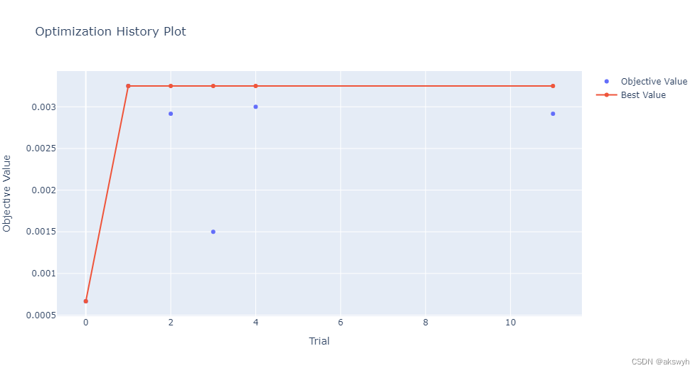
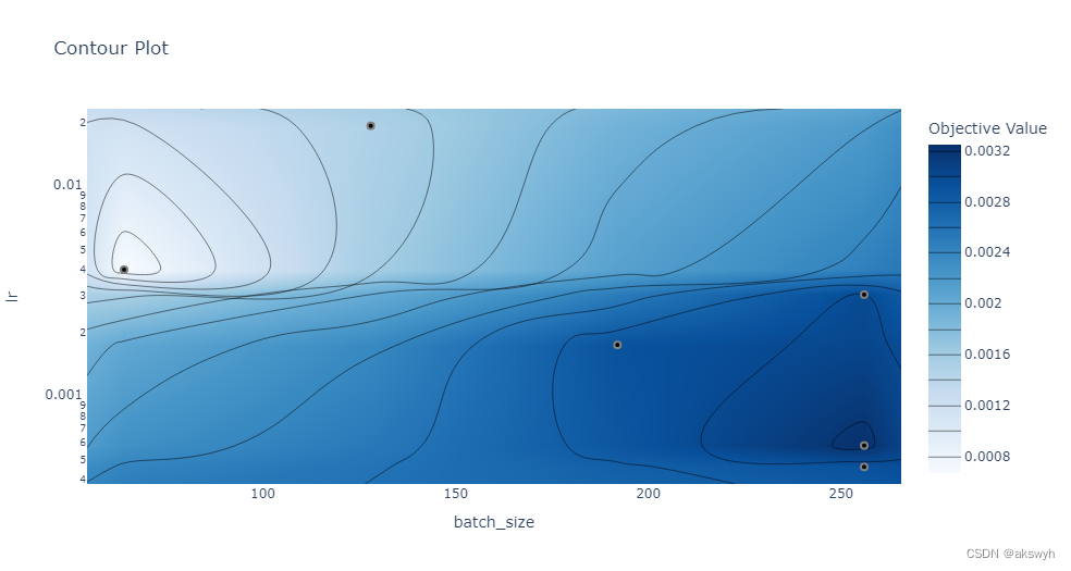
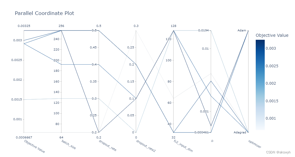
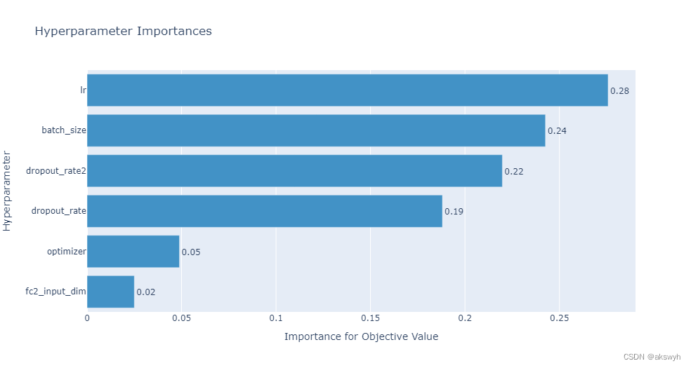
optuna寻优过程中的部分图
因为绘图用到了plotly库,在jupyter上可以直接绘制出来
optuna. visualization. plot_optimization_history( study)
optuna. visualization. plot_contour( study, params= [ 'batch_size' , 'lr' ] )
optuna. visualization. plot_parallel_coordinate( study)
optuna. visualization. plot_param_importances( study)


 1756
1756


 被折叠的 条评论
为什么被折叠?
被折叠的 条评论
为什么被折叠?
 到【灌水乐园】发言


