


研究问题:当MRC任务中涉及无法回答的问题时,除encoder外,还需要一个称为verification的基本验证模块,以MRC建模的最新实践仍然主要受益于采用经过良好训练的pre-trained LM作为encoder block,只关注“读取”。
解决方法:为了更好的探索verifier的设计,该论文提出Retrospective reader(Retro-Reader),包含两步:
- 粗略阅读,简要调查文章和问题的整体关联,并得出初步判断;
- 精细阅读,验证答案并给出最终预测。
Contributions:
-
提出了一种新的回溯式阅读器设计,它能够充分有效地进行答案验证,而不是简单地在现有阅读器中堆叠验证程序。
-
实验表明,我们的回溯阅读器可以在强大的基线上产生实质性的改进,并在基准MRC任务上获得最新的结果。
-
由于Encoder端的PreTrained LM太过于强大,所以该论文主要关注Decoder端如段落和问题-注意交互,尤其是答案验证
1. 前人工作:
- Liu et al.2018 向context中添加一个空的word token,并且最后给reader加一个简单的classification layer
- Hu et al.2019 额外使用两种不同类型的loss,独立的span loss预测可回答的问题,以及非独立的loss决定问题是否可回答,此外,还采用了一个额外的验证器来确定预测答案是否由输入的片段所包含(Figure 1-[b])
- back et al.2020 提出一个attention-based satisfaction score来比较question embedding和cacidate answer embeddings(Figure 1-[C])
- zhang et al.2020c 提出一个基于BERTverifier layer,它是一个线性层,用于context embedding,通过上下文词的表示对start和end的分布进行加权,并连接到[CLS]token表示,以进行验证
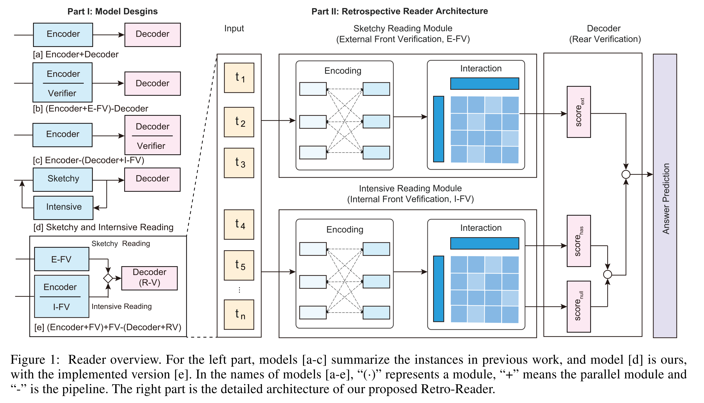
2. 该论文的模型
retrospective reader由两个并行模块组成的two-stage阅读过程:
- sketchy reading module:对于问题是否可以回答,作出一个粗略的判断(external front verifcation)
- intensive reading module:预测candidate answers,并且用answerability confidence(internal front verification)联合sketchy judgment score生成最后的答案(rear verification)
2.1 Sketchy Reading Module
2.1.1 Embedding
将question和passage texts拼接作为输入,送进encoder(如PLM)
2.1.2 Interaction
Embedding的结果经过multi-layer Transformer
h
^
i
l
+
1
=
Σ
m
=
1
M
W
m
l
+
1
{
Σ
j
=
1
n
A
i
,
j
m
⋅
V
m
l
+
1
x
j
l
}
(1)
\hat{h}_{i}^{l+1} = \Sigma_{m=1}^{M}W_m^{l+1}\{\Sigma_{j=1}^{n}A_{i,j}^m{\cdot}V_m^{l+1}x_j^l\}\tag{1}
h^il+1=Σm=1MWml+1{Σj=1nAi,jm⋅Vml+1xjl}(1)
h i l + 1 = L a y e r N o r m ( x i l + h ^ i l + 1 ) (2) h_i^{l+1} = LayerNorm(x^l_i + \hat{h}_i^{l+1})\tag{2} hil+1=LayerNorm(xil+h^il+1)(2)
x ^ i l + 1 = W 2 l + 1 ⋅ G E L U ( W 1 l + 1 h i l + 1 + b 1 l + 1 ) + b 2 l + 1 (3) \hat{x}_i^{l+1} = W_2^{l+1}{\cdot}GELU(W_1^{l+1}h_i^{l+1}+b_1^{l+1})+b_2^{l+1}\tag{3} x^il+1=W2l+1⋅GELU(W1l+1hil+1+b1l+1)+b2l+1(3)
x i l + 1 = L a y e r N o r m ( h i l + 1 + x ^ i l + 1 ) (4) x_i^{l+1} = LayerNorm(h_i^{l+1}+\hat{x}_i^{l+1})\tag{4} xil+1=LayerNorm(hil+1+x^il+1)(4)
- m是指attention heads的index
- A i , j m A_{i,j}^m Ai,jm是指 A t t e n t i o n ( Q , K , V ) = s o f t m a x ( Q K T d k ) V Attention(Q,K,V)=softmax(\frac{QK^T}{\sqrt{d_k}})V Attention(Q,K,V)=softmax(dkQKT)V前半部分,即 s o f t m a x ( Q K T d k ) softmax(\frac{QK^T}{\sqrt{d_k}}) softmax(dkQKT),有 A i , j m ∝ exp [ ( Q m l + 1 x i l ) T ( K m l + 1 x j l ) ] A_{i,j}^m\propto\exp[(Q_m^{l+1}x_i^l)^T(K_m^{l+1}x_j^l)] Ai,jm∝exp[(Qml+1xil)T(Kml+1xjl)],即 exp \exp exp后表示normalization
- W m l + 1 , Q m l + 1 , K m l + 1 , V m l + 1 W_m^{l+1},Q_m^{l+1},K_m^{l+1},V_m^{l+1} Wml+1,Qml+1,Kml+1,Vml+1都是通过 m m m-th head attention学习到的参数, W 1 l + 1 , W 2 l + 1 , b 1 l + 1 , b 2 l + 1 W_1^{l+1},W_2^{l+1},b_1^{l+1},b_2^{l+1} W1l+1,W2l+1,b1l+1,b2l+1是学习到的参数和偏置
External Front Verification(E-FV)
实际上是一个而分类任务,将第一个token([CLS])
h
1
∈
H
h_1\in{\bf H}
h1∈H送到全连接曾,做一个分类预测结果,训练的loss函数是一个交叉熵函数
L
a
n
s
=
−
1
N
Σ
i
=
1
N
[
y
i
log
y
i
^
+
(
1
−
y
i
)
log
(
1
−
y
i
^
)
]
(5)
L^{ans} = - \frac{1}{N}\Sigma^{N}_{i=1}[y_i\log\hat{y_i}+(1-y_i)\log(1-\hat{y_i})] \tag{5}
Lans=−N1Σi=1N[yilogyi^+(1−yi)log(1−yi^)](5)
计算exteranl verification得分:
s
c
o
r
e
e
x
t
=
l
o
g
i
t
n
a
−
l
o
g
i
t
a
n
s
score_{ext}=logit_{na}-logit_{ans}
scoreext=logitna−logitans
2.2 Intensive Reading Module
和sketchy reader的interaction procedure一样,获得representation H \bf H H,之前的BERT、XLNET、ALBERT都是直接将 H \bf H H直接送进线性层生成预测结果
2.2.1 Question-aware Matching
根据位置信息,将representation H \bf H H分开变成 H Q {\bf H}^Q HQ和 H P {\bf H}^P HP, 然后研究了两种潜在的question-aware matching机制
Cross Attention: Transformer-style multi-head cross attention
将 H \bf H H和 H Q {\bf H}^Q HQ送入一个revised one-layer multi-head attention layer(由Lu et al.2019提出),其中 Q = K = V \bf Q=K=V Q=K=V,将其中的 Q \bf Q Q替换成 H \bf H H, K \bf K K和 V \bf V V替换成 H Q {\bf H}^Q HQ,得到最后的表示 H ′ \bf H' H′
Matching Attention: traditional matching attention
将
H
\bf H
H和
H
Q
{\bf H}^Q
HQ送入一个传统的matching attentio层(由WANG ET AL.2017提出)
M
=
s
o
f
t
M
a
x
(
H
(
W
H
Q
+
b
⨂
e
T
)
)
{\bf M}={\rm softMax}({\bf H}({\bf WH}^Q+{{\bf b} \bigotimes{\bf e}}^T))
M=softMax(H(WHQ+b⨂eT))
H ′ = M H Q (6) {\bf H'=MH}^Q \tag{6} H′=MHQ(6)
- W \bf W W和 b \bf b b是学习的参数
- e \bf e e是一个全一向量,用于将偏差向量重复到矩阵中
- M \bf M M代表了两个序列不同的隐藏层状态的权重
- H ′ \bf H' H′是所有的隐藏层状态的权重和,代表了 H \bf H H中的向量如何与 H Q {\bf H}^Q HQ中的每一个隐藏状态对齐,并且用于最后的预测
2.2.2 Span Prediction
用一个Linear layer进行softmax,并将
H
′
\bf H'
H′作为其输入,得到开始位置和结束位置的概率
s
,
e
∝
S
o
f
t
M
a
x
(
F
F
N
(
H
′
)
)
(7)
s,e \propto \rm SoftMax(FFN(\bf H')) \tag{7}
s,e∝SoftMax(FFN(H′))(7)
训练的loss定义为
L
s
p
a
n
=
−
1
N
Σ
i
N
[
log
(
p
y
i
s
s
)
+
l
o
g
(
p
y
i
e
e
)
]
(8)
L^{span}=-\frac{1}{N}\Sigma_{i}^{N}[\log(p^s_{y^s_i})+log(p^e_{y_{i}^e})] \tag{8}
Lspan=−N1ΣiN[log(pyiss)+log(pyiee)](8)
- 其中 y i s y_i^s yis和 y i e y_i^e yie代表i样本ground-truth的开始和结束
2.2.3 Internal Front Verification(I-FV)
-
I-FV-CE
y ‾ i , k = SoftMax ( FFN ( h 1 ′ ) ) L a n s = − 1 N ∑ i = 1 N ∑ k = 1 K [ y i , k log y ‾ i , k ] (9) \overline{y}_{i,k}=\operatorname{SoftMax}(\operatorname{FFN}(h_1')) \\ L^{ans} = -\frac{1}{N}\sum_{i=1}^N\sum_{k=1}^K[y_{i,k}\log{\overline{y}}_{i,k}] \tag{9} yi,k=SoftMax(FFN(h1′))Lans=−N1i=1∑Nk=1∑K[yi,klogyi,k](9)
- K K K代表类别的数量,这里 K = 2 K=2 K=2
-
I-FV-BE
y ‾ i = Sigmoid ( FFN ( h 1 ′ ) ) L a n s = − 1 N ∑ i = 1 N [ y i log y ‾ i + ( 1 − y i ) log ( 1 − y ‾ i ) ] (10) \overline{y}_{i}=\operatorname{Sigmoid}(\operatorname{FFN}(h_1')) \\ L^{ans} = -\frac{1}{N}\sum_{i=1}^{N}[y_i\log\overline{y}_i+(1-y_i)\log(1-\overline{y}_i)] \tag{10} yi=Sigmoid(FFN(h1′))Lans=−N1i=1∑N[yilogyi+(1−yi)log(1−yi)](10)
- I-FV-MSE
y ‾ i = FFN ( h 1 ′ ) L a n s = − 1 N ∑ i = 1 N ( y i − y i ‾ ) 2 (11) \overline{y}_{i}=\operatorname{FFN}(h_1') \\ L^{ans} = -\frac{1}{N}\sum_{i=1}^{N}(y_i-\overline{y_i})^2 \tag{11} yi=FFN(h1′)Lans=−N1i=1∑N(yi−yi)2(11)
FV的联合loss function如下:
L
=
α
1
L
s
p
a
n
+
α
2
L
a
n
s
(13)
L=\alpha_1L^{span}+\alpha_2L^{ans} \tag{13}
L=α1Lspan+α2Lans(13)
2.2.4 Threshold-based Answerable Verification(TAV)
s c o r e h a s = max ( s k + e l ) , 1 < k ≤ l < n s c o r e n u l l = s 1 + e 1 s c o r e d i f f = s c o r e n u l l − s c o r e h a s (14) score_{has}=\max(s_k+e_l), 1< k \leq l < n score_{null} = s_1+e_1 \tag{14} score_{diff} = score_{null}-score_{has} scorehas=max(sk+el),1<k≤l<nscorenull=s1+e1scorediff=scorenull−scorehas(14)
2.3 Rear Verification
将E-FV和I-FV的predicted probilities拼接,
v
=
β
1
s
c
o
r
e
d
i
f
f
+
β
2
s
c
o
r
e
e
x
t
v=\beta_1score_{diff}+\beta_2score_{ext}
v=β1scorediff+β2scoreext
-
β
1
\beta_1
β1和
β
2
\beta_2
β2是权重
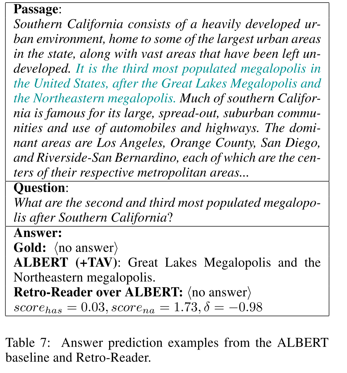
当 v > δ v > \delta v>δ, δ \delta δ是模型预测出来 h a s − a n s w e r has-answer has−answer的得分,问题有解
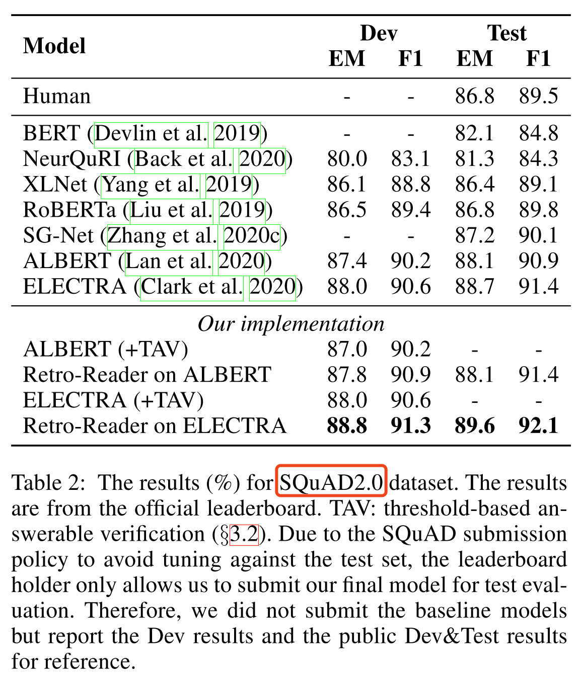
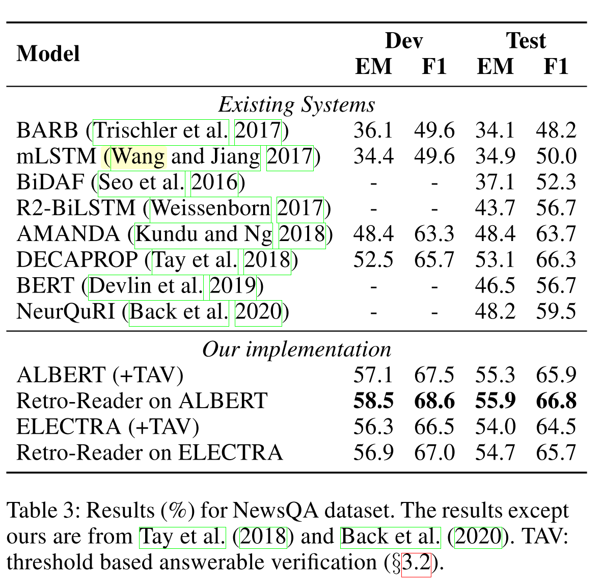
3. 实验分析
数据集:SQuAD2.0和NewsQA
模型样例:


 1323
1323


 被折叠的 条评论
为什么被折叠?
被折叠的 条评论
为什么被折叠?
 到【灌水乐园】发言


