


连续干预
econml.dml.DML — econml 0.14.1 documentation
在这个示例中,我们使用LinearDML模型,使用随机森林回归模型来估计因果效应。我们首先模拟数据,然后模型,并使用方法来effect创建不同干预值下的效应(Conditional Average Treatment Effect,CATE)。
请注意,实际情况中的数据可能更加复杂,您可能需要根据您的数据和问题来适当选择的模型和参数。此示例仅供参考,您可以根据需要进行修改和扩展。
import numpy as np
from econml.dml import LinearDML

# 生成示例数据
np.random.seed(123)
n_samples = 1000
n_features = 5
X = np.random.normal(size=(n_samples, n_features))
T = np.random.uniform(low=0, high=1, size=n_samples)  # 连续干预变量
y = 2 * X[:, 0] + 0.5 * X[:, 1] + 3 * T + np.random.normal(size=n_samples)

# 初始化 LinearDML 模型
est = LinearDML(model_y='auto', model_t='auto', random_state=123)

# 拟合模型
est.fit(y, T, X=X)

# 给定特征和连续干预值,计算干预效应
X_pred = np.random.normal(size=(10, n_features))  # 假设有新的数据点 X_pred
T_pred0 = np.array([0]*10)  # 指定的连续干预值
T_pred11 = np.array([0.2, 0.4, 0.6, 0.8, 1.0, 0.3, 0.5, 0.7, 0.9, 0.1])  # 指定的连续干预值
T_pred1 = np.array([0.2]*10)  # 指定的连续干预值
T_pred2 = np.array([0.4]*10)  # 指定的连续干预值
T_pred3 = np.array([0.6]*10)  # 指定的连续干预值
T_pred4 = np.array([0.8]*10)  # 指定的连续干预值


# 计算连续干预效应
effect_pred = est.effect(X=X_pred, T0=T_pred0, T1=T_pred11)

print("预测的连续干预效应:", effect_pred)

# 计算连续干预效应
effect_pred = est.effect(X=X_pred, T0=T_pred0, T1=T_pred1)

print("预测的连续干预效应:", effect_pred)在经济学因果推断(EconML)中,marginal_effect 和 effect 是两个不同的概念:
-
Effect(因果效应):effect通常是指一个因果估计的结果,表示一个变量(例如处理、干预、政策等)对另一个变量(例如结果、响应)的影响程度。这通常是一个定量的值,可以是正数、负数或零,用于表示处理对结果的影响,例如处理导致结果增加或减少了多少。 -
Marginal Effect(边际效应):marginal effect是指一个因果估计模型中,对一个变量进行微小变化时,对结果的影响。它表示了在其他变量保持不变的情况下,对某个特定变量进行微小变化时,对结果的影响。Marginal effect可以用来理解在不同情况下,对一个特定变量的微小变化对结果的影响。
例如,在回归模型中,effect 可能表示了某个因素对目标变量的总体影响,而 marginal effect 可能表示了在某个特定数值点上,对一个自变量进行微小变化时,目标变量的变化程度。
总之,effect 表示总体影响,而 marginal effect 表示在特定情境下,自变量微小变化对因果结果的影响。这两个概念在因果推断中经常使用,用于深入理解因果关系和模型的行为。
# 使用 final_model_ 预测因果效应
effect_pred = est.model_final_.predict(np.column_stack((T_pred1, X)))

print(effect_pred)
def effect(self, X, T0=0, T1=1):
"""
Parameters
----------
X : features
"""
if not hasattr(T0, "__len__"):
T0 = np.ones(X.shape[0])*T0
if not hasattr(T1, "__len__"):
T1 = np.ones(X.shape[0])*T1
X0 = hstack([T0.reshape(-1, 1), X])
X1 = hstack([T1.reshape(-1, 1), X])
return self.model_final.predict(X1) - self.model_final.predict(X0)
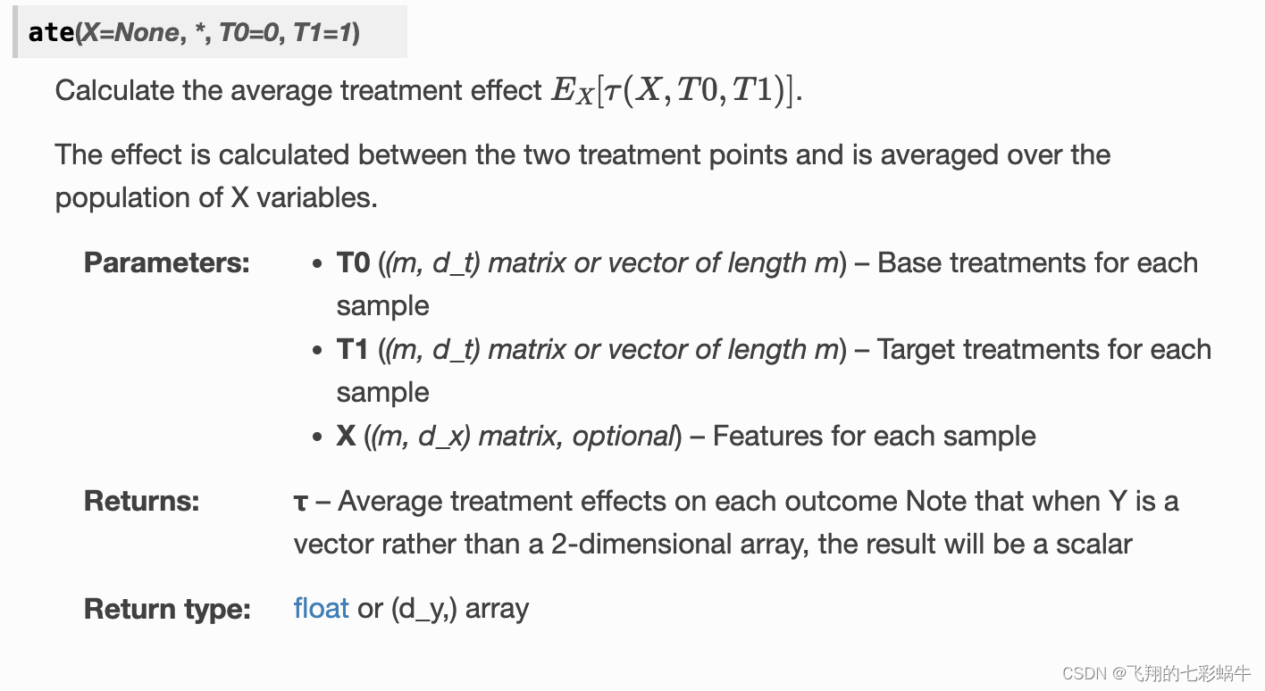
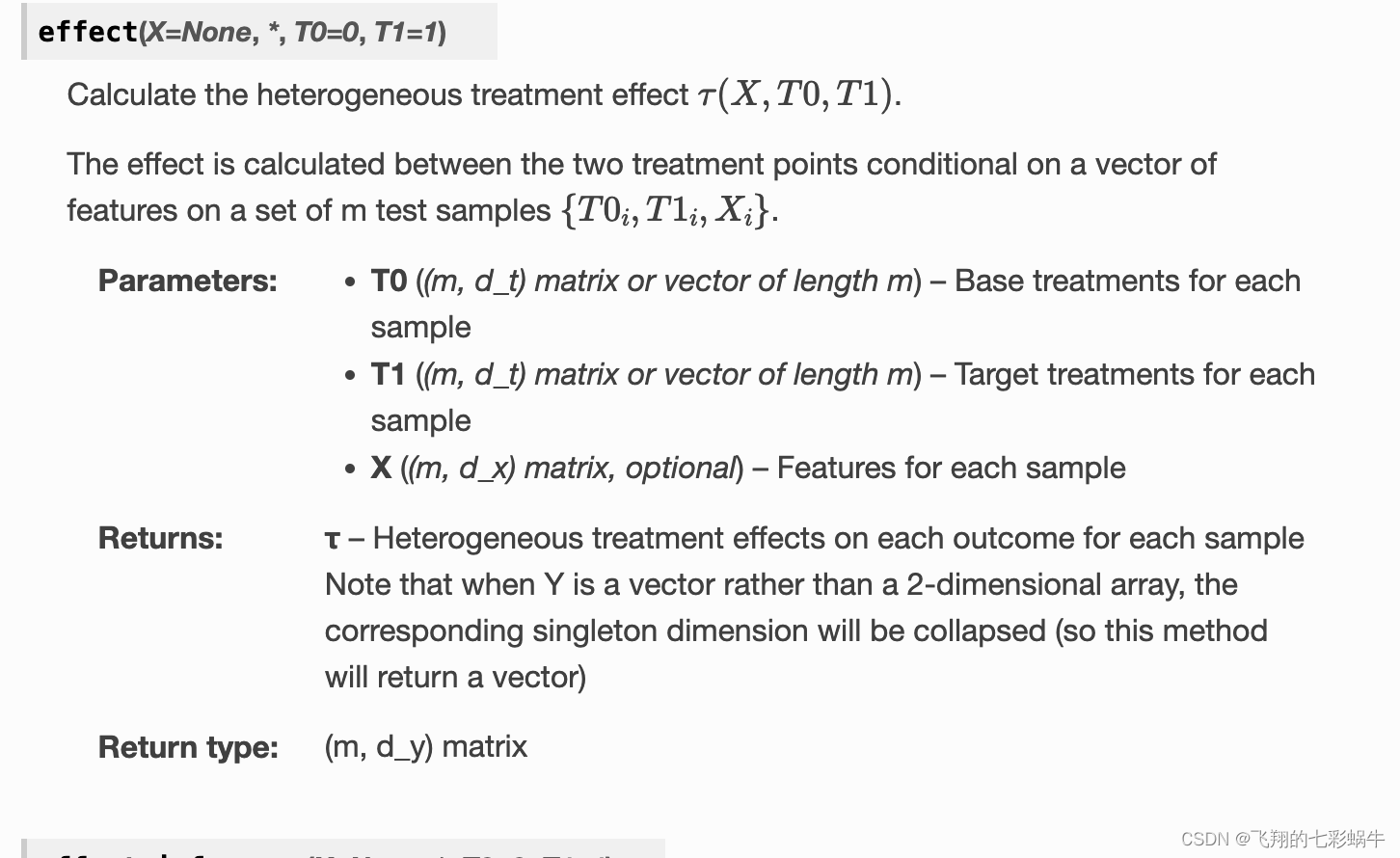
def effect(self, X=None, *, T0, T1):
"""
Calculate the heterogeneous treatment effect :math:`\\tau(X, T0, T1)`.
The effect is calculated between the two treatment points
conditional on a vector of features on a set of m test samples :math:`\\{T0_i, T1_i, X_i\\}`.
Since this class assumes a linear effect, only the difference between T0ᵢ and T1ᵢ
matters for this computation.
Parameters
----------
T0: (m, d_t) matrix
Base treatments for each sample
T1: (m, d_t) matrix
Target treatments for each sample
X: (m, d_x) matrix, optional
Features for each sample
Returns
-------
effect: (m, d_y) matrix (or length m vector if Y was a vector)
Heterogeneous treatment effects on each outcome for each sample.
Note that when Y is a vector rather than a 2-dimensional array, the corresponding
singleton dimension will be collapsed (so this method will return a vector)
"""
X, T0, T1 = self._expand_treatments(X, T0, T1)
# TODO: what if input is sparse? - there's no equivalent to einsum,
# but tensordot can't be applied to this problem because we don't sum over m
eff = self.const_marginal_effect(X)
# if X is None then the shape of const_marginal_effect will be wrong because the number
# of rows of T was not taken into account
if X is None:
eff = np.repeat(eff, shape(T0)[0], axis=0)
m = shape(eff)[0]
dT = T1 - T0
einsum_str = 'myt,mt->my'
if ndim(dT) == 1:
einsum_str = einsum_str.replace('t', '')
if ndim(eff) == ndim(dT): # y is a vector, rather than a 2D array
einsum_str = einsum_str.replace('y', '')
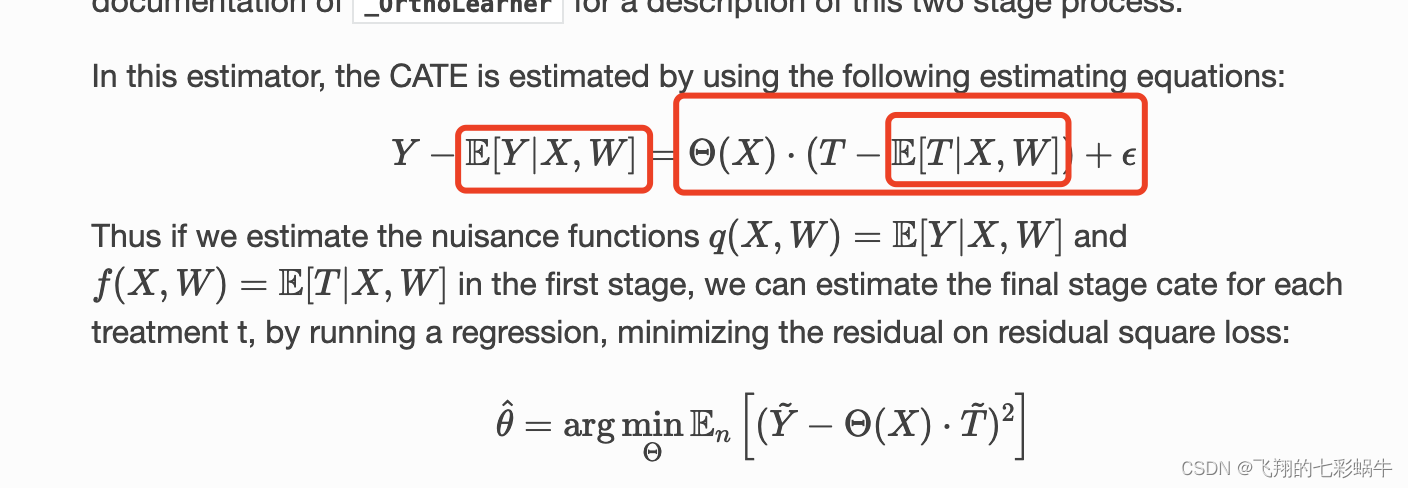
return np.einsum(einsum_str, eff, dT)The R Learner is an approach for estimating flexible non-parametric models of conditional average treatment effects in the setting with no unobserved confounders. The method is based on the idea of Neyman orthogonality and estimates a CATE whose mean squared error is robust to the estimation errors of auxiliary submodels that also need to be estimated from data:
the outcome or regression model
the treatment or propensity or policy or logging policy model
est = DML(
    model_y=RandomForestClassifier(),
    model_t=RandomForestRegressor(),
    model_final=StatsModelsLinearRegression(fit_intercept=False),
    linear_first_stages=False,
    discrete_treatment=False
)
使用随机实验数据进行双重机器学习(DML)训练可能会在某些情况下获得更好的效果,但并不是绝对的规律。DML方法的性能取决于多个因素,包括数据质量、特征选择、模型选择和调参等。
使用随机实验数据进行训练的优势在于,实验数据通常可以更好地控制混淆因素,从而更准确地估计因果效应。如果实验设计得当,并且随机化合理,那么通过DML训练的模型可以更好地捕捉因果关系,从而获得更准确的效应估计。
然而,即使使用随机实验数据,DML方法仍然需要考虑一些因素,例如样本大小、特征的选择和处理、模型的选择和调参等。在实际应用中,没有一种方法可以适用于所有情况。有时,随机实验数据可能会受到实验设计的限制,或者数据质量可能不足以获得准确的效应估计。
因此,使用随机实验数据进行DML训练可能会在某些情况下获得更好的效果,但并不是绝对的规律。在应用DML方法时,仍然需要根据实际情况进行数据分析、模型选择和验证,以确保获得准确和可靠的因果效应估计。
连续干预/label01
import numpy as np
from econml.dml import LinearDML
import scipy

# 生成示例数据
np.random.seed(123)
n_samples = 1000
n_features = 5
X = np.random.normal(size=(n_samples, n_features))
T = np.random.uniform(low=0, high=1, size=n_samples)  # 连续干预变量
#y = 2 * X[:, 0] + 0.5 * X[:, 1] + 3 * T + np.random.normal(size=n_samples)
y = np.random.binomial(1, scipy.special.expit(X[:, 0]))

# 初始化 LinearDML 模型
est = LinearDML(model_y='auto', model_t='auto', random_state=123)

# 拟合模型
est.fit(y, T, X=X)

# 给定特征和连续干预值,计算干预效应
X_pred = np.random.normal(size=(10, n_features))  # 假设有新的数据点 X_pred
T_pred0 = np.array([0]*10)  # 指定的连续干预值
T_pred11 = np.array([0.2, 0.4, 0.6, 0.8, 1.0, 0.3, 0.5, 0.7, 0.9, 0.1])  # 指定的连续干预值
T_pred1 = np.array([0.2]*10)  # 指定的连续干预值
T_pred2 = np.array([0.4]*10)  # 指定的连续干预值
T_pred3 = np.array([0.6]*10)  # 指定的连续干预值
T_pred4 = np.array([0.8]*10)  # 指定的连续干预值


# 计算连续干预效应
effect_pred = est.effect(X=X_pred, T0=T_pred0, T1=T_pred11)

print("预测的连续干预效应:", effect_pred)
预测的连续干预效应: [-0.00793674  0.00612109  0.03141778  0.00310806 -0.01635394 -0.01905434
  0.06801354 -0.0126543  -0.04603434  0.00821044]
ate是一个值
dml原理
Double Machine Learning, DML。
方法:首先通过X预测T,与真实的T作差,得到一个T的残差,然后通过X预测Y,与真实的Y作差,得到一个Y的残差,预测模型可以是任何ML模型,最后基于T的残差和Y的残差进行因果建模。
原理:DML采用了一种残差回归的思想。
优点:原理简单,容易理解。预测阶段可以使用任意ML模型。
缺点: 需要因果效应为线性的假设。
应用场景:适用于连续Treatment且因果效应为线性场景
单调性约束
因果推断的开源包中,有一些可以进行单调性约束的案例。这些案例通常涉及到因果效应的估计,同时加入了单调性约束以确保结果更加合理和可解释。以下是一些开源包以及它们支持单调性约束的案例示例:
-
CausalML(https://causalml.readthedocs.io/):
CausalML 是一个开源的因果推断工具包,支持单调性约束。它提供了一些可以用于处理单调性约束的方法,例如SingleTreatment类。您可以使用该包来在处理因果效应时添加单调性约束。
-
econml(https://econml.azurewebsites.net/):
- econml 也是一个用于因果推断的工具包,支持单调性约束。它提供了一些工具,如
SingleTreePolicyInterpreter和SingleTreeCateInterpreter,用于解释单一决策树的因果效应,并且可以根据用户指定的特征添加单调性约束。
- econml 也是一个用于因果推断的工具包,支持单调性约束。它提供了一些工具,如
SingleTreeCateInterpreter(_SingleTreeInterpreter):
    """
    An interpreter for the effect estimated by a CATE estimator

    Parameters
    ----------
    include_model_uncertainty : bool, default False
        Whether to include confidence interval information when building a
        simplified model of the cate model. If set to True, then
        cate estimator needs to support the `const_marginal_ate_inference` method.

    uncertainty_level : double, default 0.05
        The uncertainty level for the confidence intervals to be constructed
        and used in the simplified model creation. If value=alpha
        then a multitask decision tree will be built such that all samples
        in a leaf have similar target prediction but also similar alpha
        confidence intervals.

    uncertainty_only_on_leaves : bool, default True
        Whether uncertainty information should be displayed only on leaf nodes.
        If False, then interpretation can be slightly slower, especially for cate
        models that have a computationally expensive inference method.


 1万+
1万+

 被折叠的 条评论
为什么被折叠?
被折叠的 条评论
为什么被折叠?
 到【灌水乐园】发言


