


- Content
(1) Calculate the vector of mean returns and covariance matrix of returns for the ten industry portfolios. Create a table showing the mean returns and standard deviation of returns for the ten industry portfolios.
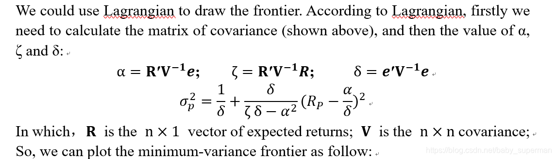
(2) Plot the minimum-variance frontier generated by the ten industry portfolios (x: standard deviation of return, range from 0% to 2%; y: mean return)
(3) Plot the efficient frontier (with the riskless asset) on the same plot
(4) Calculate the weights of the ten industry portfolios at the tangency portfolio

- code
file = 'Industry_Portfolios.xlsx'
df = pd.read_excel(file)

# describe df
df=DataFrame.drop(df,'Date',axis=1)
des=DataFrame.describe(df)

# caculate mean returns and covariance matrix of returns
table=des[1:3]

mean_return=np.mean(df,axis=0)
mean_return = np.array(mean_return/100)

covariance=np.cov(df/100,rowvar=0)
covariance=np.array(covariance)


e= np.ones(10)
rp=np.linspace(0.0013,0.02,100)
a = np.dot(np.dot(np.transpose(mean_return),(np.linalg.inv(covariance))),e)
b=  np.dot(np.dot(np.transpose(mean_return),(np.linalg.inv(covariance))),mean_return)
c= np.dot(np.dot(np.transpose(e),(np.linalg.inv(covariance))),e)
minVariance =np.sqrt(1/c+c/(b*c-a**2)*(rp-a/c)**2)


#with riskless asset
rf=0.0013
minVariance1=np.sqrt((rp-rf)**2/(b-2*a*rf+c*rf**2))

plt.plot(minVariance,rp)
plt.plot(minVariance1,rp)
plt.xlabel("variance")
plt.ylabel("Rp")
plt.legend()
plt.show
plt.savefig('tupian.png')

# Calculate the weights of the ten industry portfolios at tangency portfolio
r_tg=(a*rf-b)/(c*rf-a)
lamda=(r_tg-rf)/(b-2*a*rf+c*rf**2)
weight=lamda*np.dot(np.linalg.inv(covariance),(mean_return-rf*e))
print(weight)
result:


 3080
3080

 被折叠的 条评论
为什么被折叠?
被折叠的 条评论
为什么被折叠?
 到【灌水乐园】发言


