Caffe 初学拾遗(十二) Solver

{承接CNN学习入门，笔者在这里对Caffe官方网站上的相关介绍进行了翻译总结，欢迎大家交流指正}

本文基于此刻最新的release，Caffe-rc3：

Solver:

solver通过将前向传播的推演与反向传播的参数更新相互协调，来达到减小loss的目的。

学习过程分化为两部分，Solver监督优化目标并进行权重更新，Net计算Loss与Gradient。

Caffe的solver包括：

Stochastic Gradient Descent (type: "SGD"),
AdaDelta (type: "AdaDelta"),
Adaptive Gradient (type: "AdaGrad"),
Adam (type: "Adam"),
Nesterov’s Accelerated Gradient (type: "Nesterov") and
RMSprop (type: "RMSProp")

Solver的职责：

1.依据优化目标，逐层搭建training network用于学习，test network用于测试当前性能。

2.通过调用forward / backward以及参数更新来迭代优化目标。

3.每隔一段时间测试网络性能。

4.在优化过程中保存caffemodel与solverstate的快照。

在每轮迭代中：

1.调用前传计算output与loss。

2.调用反传计算gradient。

3.根据solver的method，将梯度值融入参数更新之中。

4.根据学习率，当前状态，solver method来更新solver state。

将网络的权值参数由刚初始化的状态调整为一个训练好的模型。

比如Caffe model，Caffe solver可以在CPU/GPU两种model下运行。

Methods:

solver method 用于解决损失函数最小化类型的优化问题。

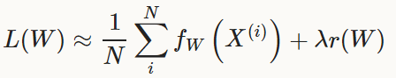
对于数据集D而言，其优化目标为全数据集|D|个数据样例的平均损失。

f_W(x(i))为数据样例x(i)的损失，r(W)是权值的正则化项，lambda是系数。

|D|的数目可能非常大，在实际操作中，我们选用随机近似的方法，选取mini-batch N << |D|，得到近似损失：

模型在前向传播中计算f_W(x)，在后向传播中计算梯度。

权值参数delta_W的更新是由误差项梯度gradient_f_W()与正则项梯度gradient_r(W)共同组成的。

SGD:

Stochastic gradient descent (type: "SGD")

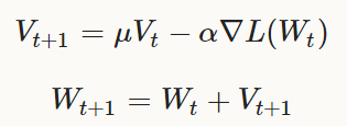
权值W的更新，是负梯度delta_L(W)和之前的权值更新结果V_t的线性组合，学习率alpha是负梯度的系数。

momentum Mu是之前的权值更新结果的系数。

形式上，我们得到如下公式用于计算在第t+1次迭代中，权值更新结果V_t+1与被更新的权重W_t+1，

已知之前的权值更新结果V_t与当前的权值W_t：

为了得到最好的结果，alpha与Mu需要进行一些微调，可以参照下文的一些方法，也可以参照：

Leon Bottou’s Stochastic Gradient Descent Tricks。

Rules of thumb for setting the learning rate α and momentum μ：

比较好的，用于深度学习的SGD策略，将学习率初始化到α≈0.01=1E−2。

当loss不再下降时，使其衰减（比如缩减为原十分之一），重复多次。

一般的，你会使用momentum μ=0.9或者类似的值，使得权值更新随着迭代过程更加平滑。

momentum 使得SGD方法下的深度学习更加稳定和迅速。

获得一个类似的学习率更新策略，你可以将如下内容加进solver prototxt文件中：

base_lr: 0.01     # begin training at a learning rate of 0.01 = 1e-2

lr_policy: "step" # learning rate policy: drop the learning rate in "steps"
                  # by a factor of gamma every stepsize iterations

gamma: 0.1        # drop the learning rate by a factor of 10
                  # (i.e., multiply it by a factor of gamma = 0.1)

stepsize: 100000  # drop the learning rate every 100K iterations

max_iter: 350000  # train for 350K iterations total

momentum: 0.9

采用上文的设定，我们在初始的100,000轮迭代中，以学习率α=0.01=1E−2开始，然后以学习率α′=αγ=(0.01)(0.1)=0.001=1E−3，

完成第100K-200K次迭代，然后以此类推，最终在350K次迭代后完成训练(max_iter)，学习率降为α‴=1E−5。

｛译者注：下一段翻译译者水平有限，可能有理解错误，敬请核查原文｝

请注意，momentum 设定为μ，在多轮迭代之后，实际上对权值的更新值V乘了系数1/(1-Mu)。如果增加Mu的话，

相应的减小alpha是一个好方法。反之亦然。

举个例子，设定Mu=0.9，实际上乘子是10，如果我们将Mu提升为0.99，乘子相应增加为100，那么我们需要将drop的因子设定为10。

即学习率alpha的衰减系数为0.1。｛译者注，更新V时的后项由于衰减0.1,100*0.1=10，仍维持后项缩放系数不变。｝

Note：

上文的方法只是一些参考，并不能保证在所有情况收敛到最优（甚至可能完全失效）。

如果训练过程发散了，请尝试降低学习率，然后重新训练，直到发现起作用的lr。

AdaDelta:

AdaDelta(type: "AdaDelta")

是一种健壮的学习率更新方法，也是一种基于梯度的最优化方案（like SGD）。

更新式为：

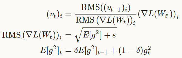
 以及：

AdaGrad:

adaptive gradient (type: "AdaGrad") 

这种基于梯度的最优化方案类似于“吹尽黄沙始见金”，发现一些预见性的但不显见的特征。

参考了之前所有迭代中的更新信息：

t′∈{1,2,...,t}

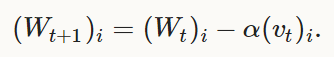
更新式为下式，权值W中的每一个元素下标为i：

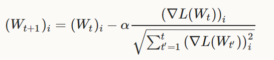
Note：

在实际操作中，权值W∈R^d，AdaGrad实现的用于存储历史梯度信息的额外存储空间是O(d)的（而不是O(dt)，

将每一次的迭代的历史梯度信息分别记录）。

Adam:

Adam (type: "Adam")

也是一种基于梯度的最优化方案（like SGD），其中包括“自适应矩估计法”(m_t,v_t)，可以被认为是泛化的AdaGrad方法:

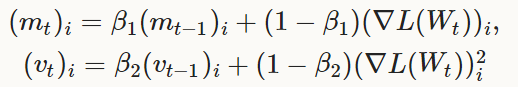
以及：

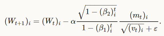
文献中取：β1=0.9,β2=0.999,ε=1E−8为初始值，Caffe中可以通过分别指定：momemtum, momentum2, delta，

来对应于β1,β2,ε。

Scaffolding:

Solver::Presolve()

准备优化算法并初始化网络模型：

> caffe train -solver examples/mnist/lenet_solver.prototxt
I0902 13:35:56.474978 16020 caffe.cpp:90] Starting Optimization
I0902 13:35:56.475190 16020 solver.cpp:32] Initializing solver from parameters:
test_iter: 100
test_interval: 500
base_lr: 0.01
display: 100
max_iter: 10000
lr_policy: "inv"
gamma: 0.0001
power: 0.75
momentum: 0.9
weight_decay: 0.0005
snapshot: 5000
snapshot_prefix: "examples/mnist/lenet"
solver_mode: GPU
net: "examples/mnist/lenet_train_test.prototxt"

Net initialization：

I0902 13:35:56.655681 16020 solver.cpp:72] Creating training net from net file: examples/mnist/lenet_train_test.prototxt
[...]
I0902 13:35:56.656740 16020 net.cpp:56] Memory required for data: 0
I0902 13:35:56.656791 16020 net.cpp:67] Creating Layer mnist
I0902 13:35:56.656811 16020 net.cpp:356] mnist -> data
I0902 13:35:56.656846 16020 net.cpp:356] mnist -> label
I0902 13:35:56.656874 16020 net.cpp:96] Setting up mnist
I0902 13:35:56.694052 16020 data_layer.cpp:135] Opening lmdb examples/mnist/mnist_train_lmdb
I0902 13:35:56.701062 16020 data_layer.cpp:195] output data size: 64,1,28,28
I0902 13:35:56.701146 16020 data_layer.cpp:236] Initializing prefetch
I0902 13:35:56.701196 16020 data_layer.cpp:238] Prefetch initialized.
I0902 13:35:56.701212 16020 net.cpp:103] Top shape: 64 1 28 28 (50176)
I0902 13:35:56.701230 16020 net.cpp:103] Top shape: 64 1 1 1 (64)
[...]
I0902 13:35:56.703737 16020 net.cpp:67] Creating Layer ip1
I0902 13:35:56.703753 16020 net.cpp:394] ip1 <- pool2
I0902 13:35:56.703778 16020 net.cpp:356] ip1 -> ip1
I0902 13:35:56.703797 16020 net.cpp:96] Setting up ip1
I0902 13:35:56.728127 16020 net.cpp:103] Top shape: 64 500 1 1 (32000)
I0902 13:35:56.728142 16020 net.cpp:113] Memory required for data: 5039360
I0902 13:35:56.728175 16020 net.cpp:67] Creating Layer relu1
I0902 13:35:56.728194 16020 net.cpp:394] relu1 <- ip1
I0902 13:35:56.728219 16020 net.cpp:345] relu1 -> ip1 (in-place)
I0902 13:35:56.728240 16020 net.cpp:96] Setting up relu1
I0902 13:35:56.728256 16020 net.cpp:103] Top shape: 64 500 1 1 (32000)
I0902 13:35:56.728270 16020 net.cpp:113] Memory required for data: 5167360
I0902 13:35:56.728287 16020 net.cpp:67] Creating Layer ip2
I0902 13:35:56.728304 16020 net.cpp:394] ip2 <- ip1
I0902 13:35:56.728333 16020 net.cpp:356] ip2 -> ip2
I0902 13:35:56.728356 16020 net.cpp:96] Setting up ip2
I0902 13:35:56.728690 16020 net.cpp:103] Top shape: 64 10 1 1 (640)
I0902 13:35:56.728705 16020 net.cpp:113] Memory required for data: 5169920
I0902 13:35:56.728734 16020 net.cpp:67] Creating Layer loss
I0902 13:35:56.728747 16020 net.cpp:394] loss <- ip2
I0902 13:35:56.728767 16020 net.cpp:394] loss <- label
I0902 13:35:56.728786 16020 net.cpp:356] loss -> loss
I0902 13:35:56.728811 16020 net.cpp:96] Setting up loss
I0902 13:35:56.728837 16020 net.cpp:103] Top shape: 1 1 1 1 (1)
I0902 13:35:56.728849 16020 net.cpp:109]     with loss weight 1
I0902 13:35:56.728878 16020 net.cpp:113] Memory required for data: 5169924

Loss：

I0902 13:35:56.728893 16020 net.cpp:170] loss needs backward computation.
I0902 13:35:56.728909 16020 net.cpp:170] ip2 needs backward computation.
I0902 13:35:56.728924 16020 net.cpp:170] relu1 needs backward computation.
I0902 13:35:56.728938 16020 net.cpp:170] ip1 needs backward computation.
I0902 13:35:56.728953 16020 net.cpp:170] pool2 needs backward computation.
I0902 13:35:56.728970 16020 net.cpp:170] conv2 needs backward computation.
I0902 13:35:56.728984 16020 net.cpp:170] pool1 needs backward computation.
I0902 13:35:56.728998 16020 net.cpp:170] conv1 needs backward computation.
I0902 13:35:56.729014 16020 net.cpp:172] mnist does not need backward computation.
I0902 13:35:56.729027 16020 net.cpp:208] This network produces output loss
I0902 13:35:56.729053 16020 net.cpp:467] Collecting Learning Rate and Weight Decay.
I0902 13:35:56.729071 16020 net.cpp:219] Network initialization done.
I0902 13:35:56.729085 16020 net.cpp:220] Memory required for data: 5169924
I0902 13:35:56.729277 16020 solver.cpp:156] Creating test net (#0) specified by net file: examples/mnist/lenet_train_test.prototxt

Completion：

I0902 13:35:56.806970 16020 solver.cpp:46] Solver scaffolding done.
I0902 13:35:56.806984 16020 solver.cpp:165] Solving LeNet

Updating Parameters：

实际上权值更新是由solver执行的，并运用在调用Solver::ComputeUpdateValue()时完成对网络参数的更新。

ComputeUpdateValue()将权值的损失项r(W)｛译者注，即loss函数中包含的lambda||W||^2项｝并入权值梯度一同计算，得到对应于每一个权值的最终梯度。这些存储在blob的diff内的梯度信息通过学习率alpha放缩，用于在Blob::Update方法调用时，通过data-diff的方式，完成最终的更新。

Snapshotting and Resuming:

Solver通过函数Solver::Snapshot()和Solver::SnapshotSolverState()，存储网络权值以及此刻状态的快照。

权值的快照导出了网络模型，而solver的快照使得从任意时刻恢复训练成为可能，训练可以通过调用Solver::Restore()以及Solver::RestoreSolverState()进行恢复。

权值文件以.caffemodel扩展名结尾，状态文件以.solverstate扩展名结尾。

两种文件在文件名中都以_iter_N形式说明迭代的轮数。

Snapshotting 配置为:

# The snapshot interval in iterations.
snapshot: 5000
# File path prefix for snapshotting model weights and solver state.
# Note: this is relative to the invocation of the `caffe` utility, not the
# solver definition file.
snapshot_prefix: "/path/to/model"
# Snapshot the diff along with the weights. This can help debugging training
# but takes more storage.
snapshot_diff: false
# A final snapshot is saved at the end of training unless
# this flag is set to false. The default is true.
snapshot_after_train: true

在solver.prototxt文件中定义。