深度学习笔记03-Pytorch实现天气识别

本文通过pytorch实现了天气识别，并完成了预测任务。

---

前言

本文为🔗365天深度学习训练营 中的学习记录博客

原作者：K同学啊

---

一、导入相关库

import torch
import torch.nn as nn
import torchvision.transforms as transforms
import torchvision
from torchvision import transforms, datasets

import os
import PIL
import pathlib
import random

device = torch.device("cuda" if torch.cuda.is_available() else "cpu")

二、导入数据

1.可视化图像

root_dir = os.getcwd()  # 获取当前工作目录
data_dir = os.path.join(root_dir, 'weather_photos')

data_dir = pathlib.Path(data_dir)

data_paths = list(data_dir.glob('*'))
classNames = [str(path).split("\\")[-1] for path in data_paths]

1. os.getcwd()获取当前工作目录当作根目录，然后用join与weather_photos拼接，得到数据目录。
2. 使用pathlib.Path()函数将字符串类型的文件夹路径转换为pathlib.Path对象。
3. 使用glob()方法获取data_dir路径下所有文件路径，并以列表形式存储在data_paths中。
4. 将文件路径转换为str类型，再通过split()函数进行分割，注意要使用’\'来分割，得到每个文件所属的类别名称，存储在classNames中。
   
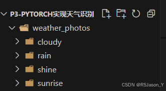
   上图是我的工作目录，天气图片一共分为cloudy、rain、shine、sunrise四种。

image_count = len(list(data_dir.glob('*/*.jpg')))
print("图片总数为：",image_count)

一共是1125张天气照片。
然后将cloudy的图片可视化，设置3行8列共展示24张图片。

import matplotlib.pyplot as plt
from PIL import Image
# 查看cloudy图像
# 指定cloudy图像文件夹路径
image_folder_cloudy = os.path.join(data_dir, 'cloudy')
image_files_cloudy = [f for f in os.listdir(image_folder_cloudy) if f.endswith((".jpg",".png",".jpeg"))]
# 创建matplotlib画布
fig, axes = plt.subplots(3, 8, figsize=(16, 6))
'''axes通常是一个由subplots() 创建的二维数组,代表多个子图的轴。
.flat属性将二维数组展平成一维迭代器，
方便逐一访问每个子图轴。'''
# 使用列表推导式加载和显示图像
for ax, img_file in zip(axes.flat, image_files_cloudy): 
    img_path = os.path.join(image_folder_cloudy, img_file)
    img = Image.open(img_path) # 打开图像文件
    ax.imshow(img) 
    ax.axis('off') # 关闭图像坐标轴
# 显示图像
plt.tight_layout() # 调整图像边界
plt.show()

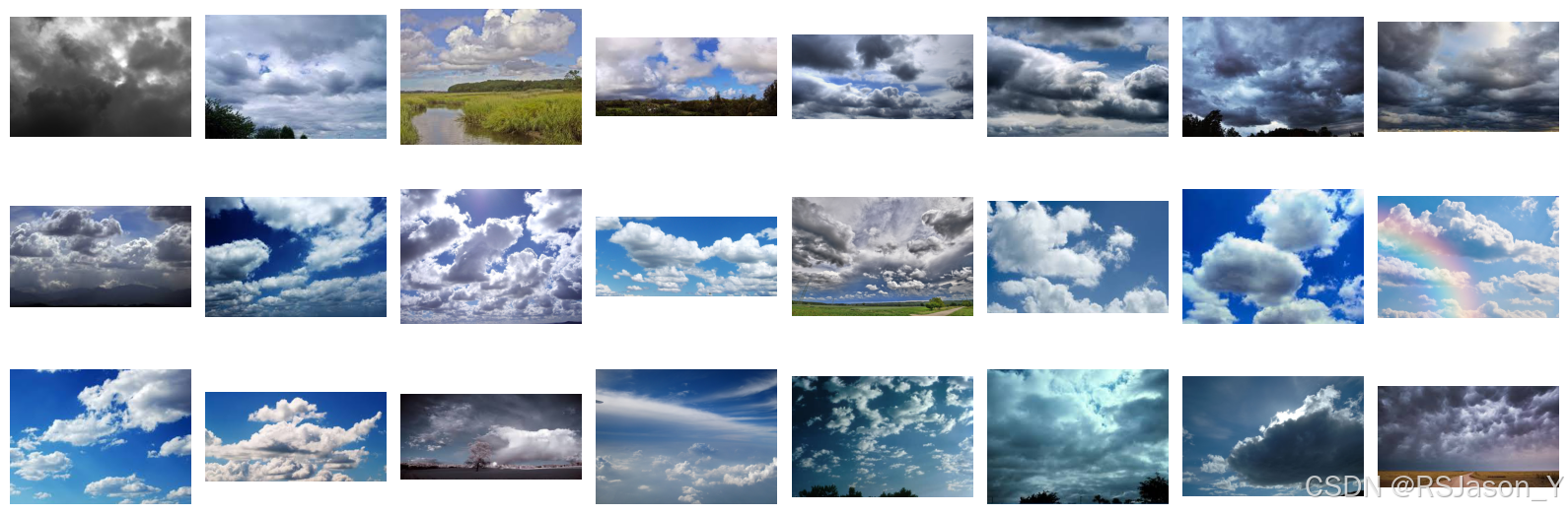
注意：axes通常是一个由subplots()创建的二维数组，代表多个子图的轴。而.flat属性将二维数组展平成一维迭代器，方便逐一访问每个子图轴。

2. 自定义transforms

代码如下（示例）：

total_datadir = os.path.join(root_dir, 'weather_photos')
# 关于transforms.Compose更多可以参考https://blog.csdn.net/qq_38251616/article/details/124878863
train_transforms = transforms.Compose([
    transforms.Resize([224, 224]), # 将输入图片resize成统一尺寸
    transforms.RandomHorizontalFlip(), # 随机水平翻转图片
    transforms.ToTensor(), # 将PIL Image或numpy.ndarray转换为tensor,并归一化到[0,1]之间
    transforms.Normalize(  # 标准化处理>=转换为标准正态分布，使模型更容易收敛
        mean = [0.485, 0.456, 0.225],
        std = [0.229, 0.224, 0.225] # 其中mean和std为ImageNet数据集的均值和方差，从数据集中随机抽样计算得到的
    )
])
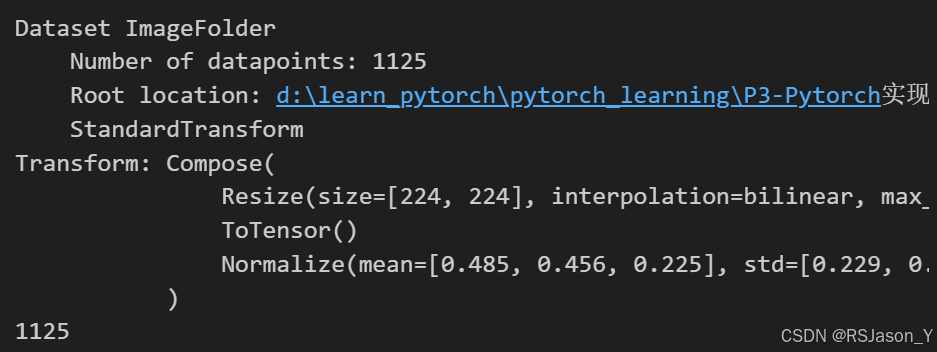
total_data = datasets.ImageFolder(root=total_datadir, transform=train_transforms)
print(total_data)
print(len(total_data))

1. Resize()是将输入图片resize成统一尺寸。
2. RandomHorizontalFlip()随机水平翻转图片。
3. ToTensor()将PIL Image或numpy.ndarray转换为tensor类型，并归一化[0,1]之间。
4. Normalize()是标准化，其中均值和标准差是ImageNet数据集的均值和方差，从数据集中随机抽样计算得到的
5. 最后通过ImageFolder()函数加载数据集。

三、加载数据集

train_size = int(0.8 * len(total_data))
test_size = len(total_data) - train_size
train_dataset, test_dataset = torch.utils.data.random_split(total_data, [train_size, test_size])
train_dataset, test_dataset

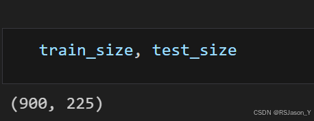
1. 将数据集按照8：2的比例划分为训练集和测试集。
2. 使用torch.utils.data.random_split()函数进行数据集划分。将total_data按照指定比例([train_size, test_size])随机划分为训练集和测试集。

batch_size = 32
train_dl = torch.utils.data.DataLoader(train_dataset, batch_size=batch_size, shuffle=True)
test_dl = torch.utils.data.DataLoader(test_dataset, batch_size=batch_size, shuffle=False)

然后使用DataLoader加载数据集，批次大小设置为32。

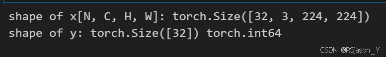
for x,y in test_dl:
    print('shape of x[N, C, H, W]:', x.shape)
    print('shape of y:', y.shape, y.dtype)
    break

四、创建CNN

import torch.nn.functional as F

class Network_bn(nn.Module):
    def __init__(self):
        super(Network_bn, self).__init__()
        self.conv1 = nn.Conv2d(3, 12, kernel_size=5, stride=1, padding=0)
        self.bn1 = nn.BatchNorm2d(12)
        self.conv2 = nn.Conv2d(12, 12, kernel_size=5, stride=1, padding=0)
        self.bn2 = nn.BatchNorm2d(12)
        self.pool1 = nn.MaxPool2d(kernel_size=2, stride=2)
        self.conv3 = nn.Conv2d(12, 24, kernel_size=5, stride=1, padding=0)
        self.bn3 = nn.BatchNorm2d(24)
        self.conv4 = nn.Conv2d(24, 24, kernel_size=5, stride=1, padding=0)
        self.bn4 = nn.BatchNorm2d(24)
        self.pool2 = nn.MaxPool2d(kernel_size=2, stride=2)
        self.fc1 = nn.Linear(24*50*50, len(classNames))


    def forward(self, x):
        x = F.relu(self.bn1(self.conv1(x)))
        x = F.relu(self.bn2(self.conv2(x)))
        x = self.pool1(x)
        x = F.relu(self.bn3(self.conv3(x)))
        x = F.relu(self.bn4(self.conv4(x)))
        x = self.pool2(x)
        x = x.view(-1, 24*50*50)
        x = self.fc1(x)

        return x

print('using {} device'.format(device))
model = Network_bn().to(device)
model

网络结构如下图所示：

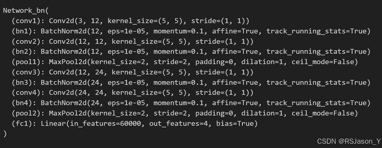
最后全连接层将60000features直接降维到classNames数量，本来写了两个全连接层，先从60000降到512，再从512降到classNames，但发现效果并不好。

五、模型训练

先设置一些超参数。

loss_fn = nn.CrossEntropyLoss()
learning_rate = 1e-4
optimizer = torch.optim.SGD(model.parameters(), lr=learning_rate)

epochs = 50
train_loss_list = []
train_acc_list = []
test_loss_list =  []
test_acc_list = []

for epoch in range(epochs):
    model.train()
    train_loss, train_acc = 0, 0
    for batch_idx, (x, y) in enumerate(train_dl):
        x, y = x.to(device), y.to(device)
        pred = model(x)
        loss = loss_fn(pred, y)
        optimizer.zero_grad()
        loss.backward()
        optimizer.step()

        train_acc += (pred.argmax(1) == y).type(torch.float).sum().item()
        train_loss += loss.item()

        if batch_idx % 10 == 0:
            loss, step = loss.item(), batch_idx
            print(f"Epoch:{epoch+1:2d}, step:[{step:1d}/{len(train_dl):1d}], running_loss: {loss:>7f}")
    
    train_acc /= len(train_dl.dataset)
    train_loss /= len(train_dl)
    train_acc_list.append(train_acc)
    train_loss_list.append(train_loss)

    model.eval()
    test_acc, test_loss = 0, 0
    with torch.no_grad():
        for batch_idx, (x, y) in enumerate(test_dl):
            x, y = x.to(device), y.to(device)
            pred = model(x)
            loss = loss_fn(pred, y)

            test_loss += loss.item()
            test_acc += (pred.argmax(1) == y).type(torch.float).sum().item()
    
    test_acc /= len(test_dl.dataset)
    test_loss /= len(test_dl)
    test_acc_list.append(test_acc)
    test_loss_list.append(test_loss)

    template = ('Epoch:{:2d}, Train_acc:{:.1f}%, Train_loss:{:.3f}, Test_acc:{:.1f}%，Test_loss:{:.3f}')
    print(template.format(epoch+1, train_acc*100, train_loss, test_acc*100, test_loss))
print('Done')

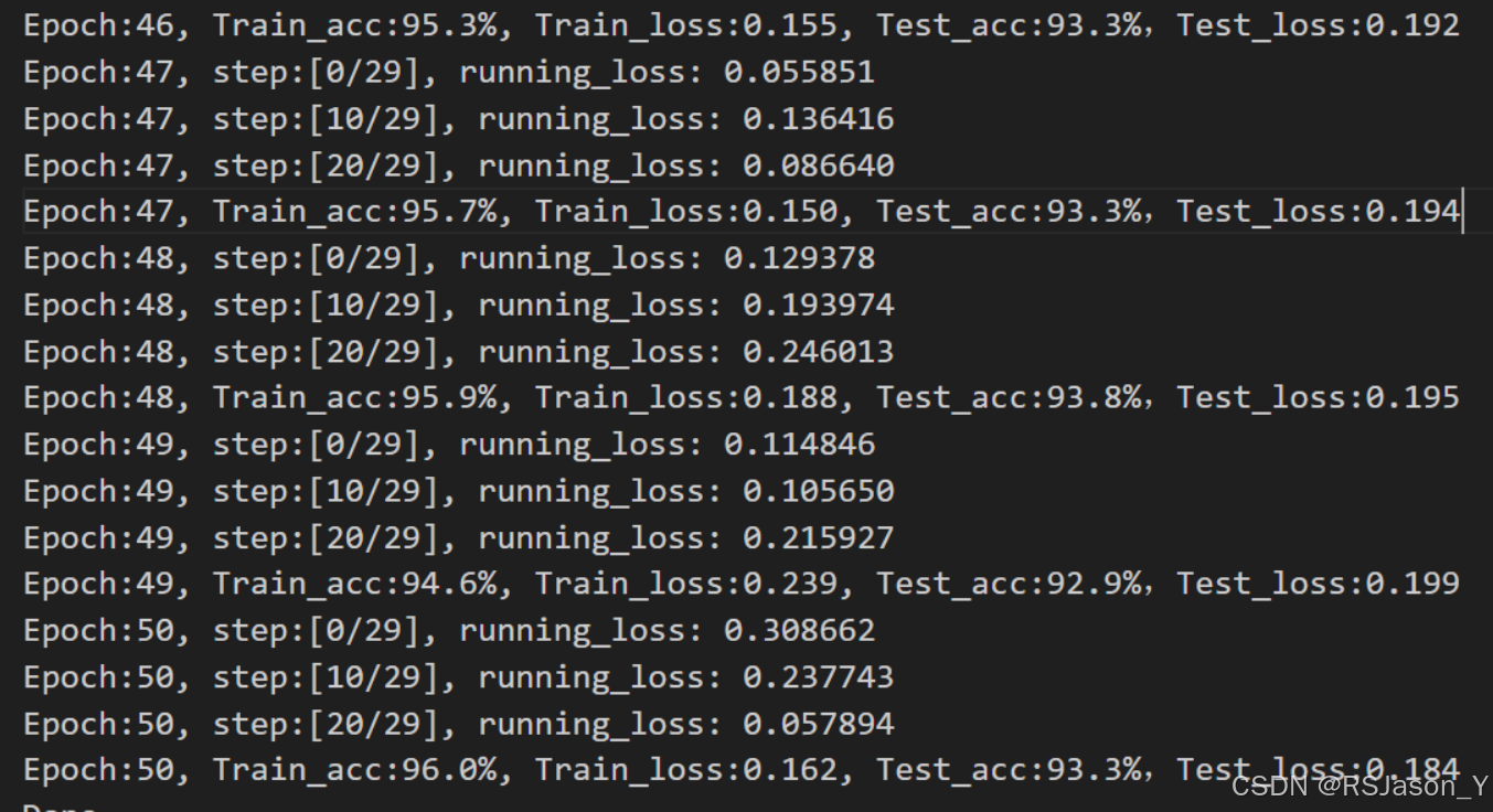
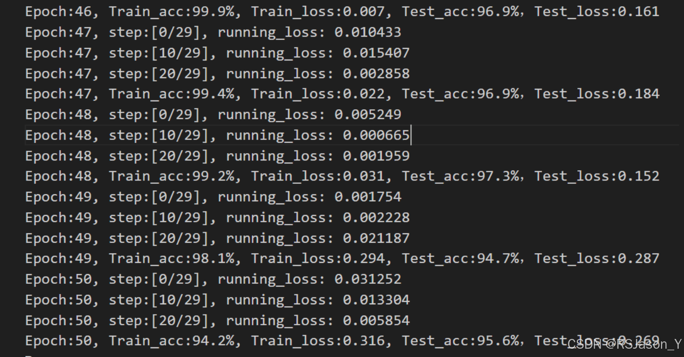
1. epoch设置为50，由于训练集一共有39个批次，因此设置每隔10个批次打印一次日志信息。
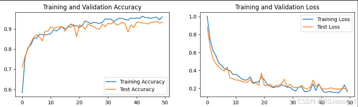
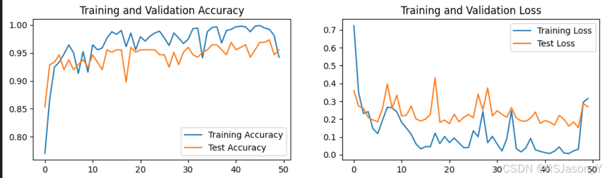
2. 本文用SGD和Adam优化器分别训练模型，发现Adam收敛速度很快，一般第一个epoch测试集准确率就能到达90多，但是它loss和准确率波动较大，并不稳定；相反，SGD虽然收敛慢一些，但总体来看，比较稳定。
3. 在50个epoch中，Adam测试集准确率最高能到97.3%，而SGD最高到93.8%。
   下图是SGD结果：
   
   
   下图是Adam结果：
   
   

六、预测

import json

weather_list = total_data.class_to_idx
cla_dict = dict((val, key) for key, val in weather_list.items())
# write dict into json file
json_str = json.dumps(cla_dict, indent=4)
with open('class_indices.json', 'w') as json_file:
    json_file.write(json_str)

# load image
img_path = './sunrise.jpg'
img = Image.open(img_path)
plt.imshow(img)
#[N,C,H,W]
img = train_transforms(img)
# expand batch dimension
img = torch.unsqueeze(img, dim=0)

# read class_indict
json_path = './class_indices.json'
with open(json_path, "r") as f:
    class_indict = json.load(f)

model = Network_bn().to(device)

# prediction
model.eval()
with torch.no_grad():
    output = torch.squeeze(model(img.to(device)))
    predict = torch.softmax(output, dim=0)
    predict_cla = torch.argmax(predict).cpu().numpy()

print_res = "class:{} prob:{:.3}".format(class_indict[str(predict_cla)],
                                             predict[predict_cla].cpu().numpy())
plt.title(print_res)
for i in range(len(predict)):
    print("class:{:10} prob:{:.3}".format(class_indict[str(i)],
                                              predict[i].cpu().numpy()))
plt.show()

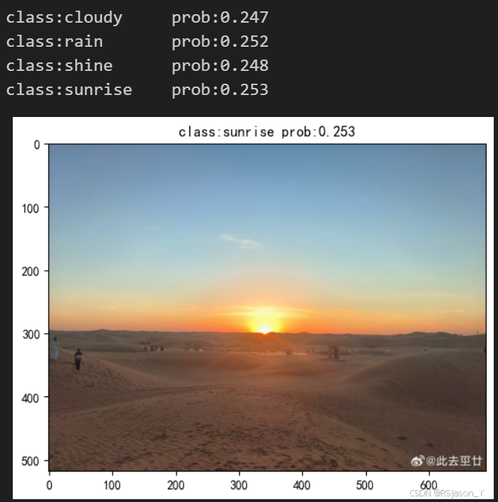
从网上随机选取了一张sunrise图片，进行预测。

1. 首先将tota_data转换为class_to_idx，也就是类别：索引类型， 然后将key,value逆转过来，生成类别字典，也就是索引：类别。
2. 将字典写成json文件。如下图所示：
   
3. 读入要预测的图片，通过自定义的transforms操作，再扩充它的batch维度，变成[batchsize, channel, height, weight]。
4. 将模型的输出通过softmax，得到预测概率值，然后再通过argmax找到概率最大值，获取预测类别。
   

---

总结

1. 完成了本地读取天气数据集，并加载数据集。
2. 测试集的准确率达到了95%以上。
3. 能够调用训练好的模型来预测一张未知的天气图片。