KNN分类和基于支持向量机的分类预测

KNN分类和基于支持向量机的分类预测

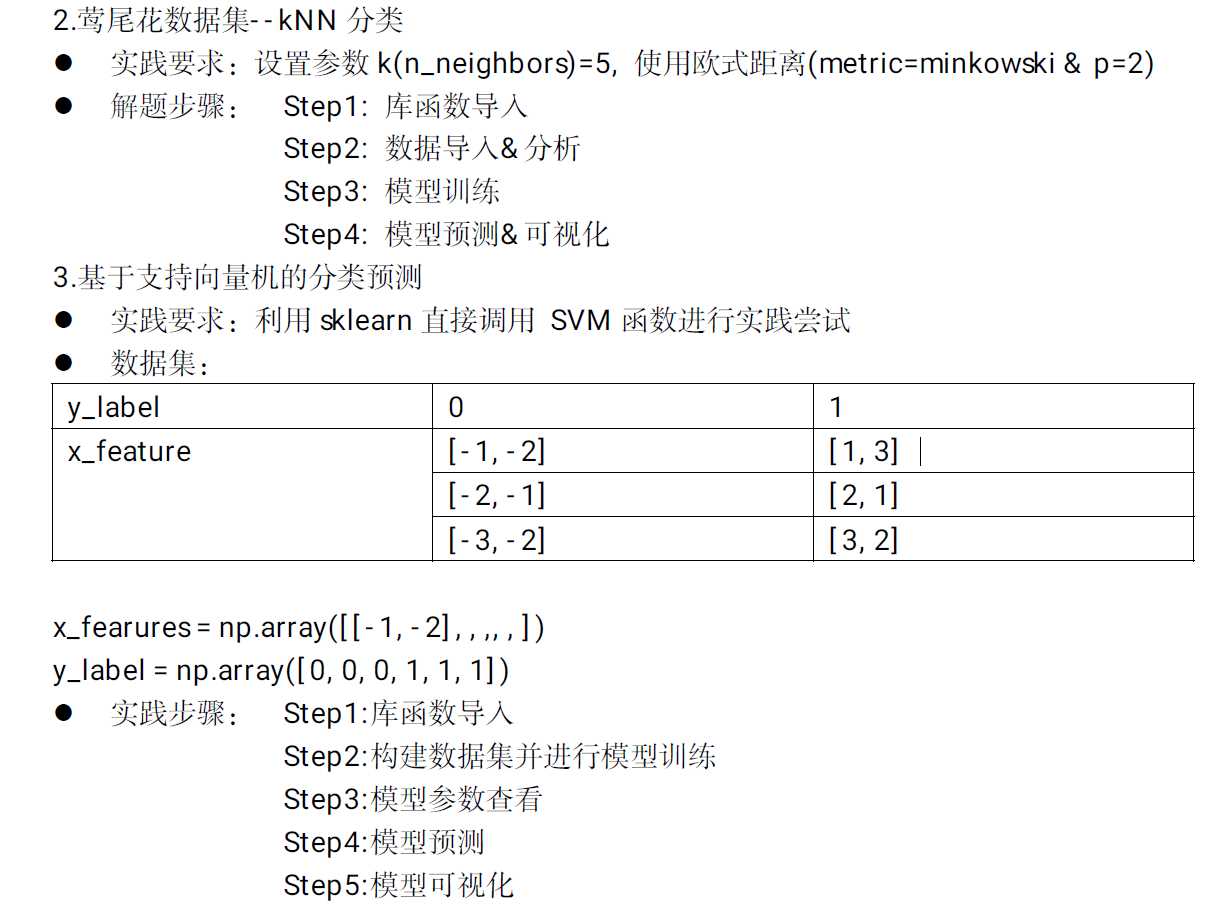
鸢尾花数据集——KNN分类

KNN分类

理解：计算未知样本与所有已知样本的距离，从中选取与未知样本距离最近的K个已知样本，根据少数服从多数的投票法则（majority-voting），将未知样本与K个最邻近样本中所属类别占比较多的归为一类。

import pandas as pd
import matplotlib.pyplot as plt
import seaborn as sns
from sklearn.datasets import load_iris
data=load_iris()
iris_target=data.target
iris_features = pd.DataFrame(data=data.data, columns=data.feature_names)  
# 利用Pandas转化为DataFrame格式


from sklearn.model_selection import train_test_split
from sklearn.neighbors import KNeighborsClassifier
from sklearn import metrics
# 为了正确评估模型性能，将数据划分为训练集和测试集，并在训练集上训练模型，在测试集上验证模型性能。
x_train, x_test, y_train, y_test = train_test_split(iris_features, iris_target,random_state=2020)
## 定义 knn模型
knn = KNeighborsClassifier(n_neighbors=5,metric='minkowski')#取最近的五个样本 使用欧几里得距离
# 在训练集上训练knn模型
knn.fit(x_train, y_train)

## 在训练集和测试集上分别利用训练好的模型进行预测
train_predict = knn.predict(x_train)
test_predict = knn.predict(x_test)

## 利用accuracy（准确度）【预测正确的样本数目占总预测样本数目的比例】评估模型效果
print('准确度:', metrics.accuracy_score(y_train, train_predict))
print('准确度:', metrics.accuracy_score(y_test, test_predict))
## 查看混淆矩阵
confusion_matrix_result = metrics.confusion_matrix(test_predict, y_test)
print('混淆矩阵结果：\n', confusion_matrix_result)

plt.figure(figsize=(8, 6))  # 指定figure的宽和高，单位为英寸
sns.heatmap(confusion_matrix_result, annot=True, cmap='Blues')
plt.xlabel('Predictedlabels')
plt.ylabel('Truelabels')
plt.show()

准确度: 0.9821428571428571
准确度: 0.9210526315789473
混淆矩阵结果：
[[15 0 0]
[ 0 10 2]
[ 0 1 10]]

基于支持向量机的分类预测

svm的理解：构造一个划分超平面，使得到两类样本点到平面的距离最大（即达到最大间隔）

sklearn.svm.SVC(C=1.0, kernel='rbf', degree=3, gamma='auto', coef0=0.0, shrinking=True, probability=False, tol=0.001, cache_size=200, class_weight=None, verbose=False, max_iter=-1, decision_function_shape=None,random_state=None)

C：C-SVC的惩罚参数C 默认值是1.0
C越大，相当于惩罚松弛变量，希望松弛变量接近0，即对误分类的惩罚增大，趋向于对训练集全分对的情况，这样对训练集测试时准确率很高，但泛化能力弱。C值小，对误分类的惩罚减小，允许容错，将他们当成噪声点，泛化能力较强。

• kernel ：核函数，默认是rbf，可以是‘linear’, ‘poly’, ‘rbf’, ‘sigmoid’, ‘precomputed’

  • 线性：u’v

  • 多项式：(gamma*u’v + coef0)^ degree

  • sigmoid：tanh(gammau’*v + coef0)

  • RBF函数: e^(-gamma|u-v|2)

• degree ：多项式poly函数的维度，默认是3，选择其他核函数时会被忽略。

• gamma ： ‘rbf’,‘poly’ 和‘sigmoid’的核函数参数。默认是’auto’，则会选择1/n_features

• coef0 ：核函数的常数项。对于‘poly’和 ‘sigmoid’有用。

• probability ：是否采用概率估计.默认为False
  布尔类型，可选，默认为False
  决定是否启用概率估计。需要在训练fit()模型时加上这个参数，之后才能用相关的方法：predict_proba和predict_log_proba

• shrinking ：是否采用shrinking heuristic方法，默认为true

• tol ：停止训练的误差值大小，默认为1e-3

• cache_size ：核函数cache缓存大小，默认为200

• class_weight ：类别的权重，字典形式传递。设置第几类的参数C为weight*C(C-SVC中的C)

• verbose ：是否允许冗余输出

• max_iter ：最大迭代次数。-1为无限制。

• decision_function_shape ：‘ovo’, ‘ovr’ or None, default=None3

• random_state ：数据洗牌时的种子值，int值

import matplotlib.pyplot as plt
import numpy as np
from sklearn import svm

x_fearures=np.array([[-1, -2], [-2, -1], [-3, -2], [1, 3], [2, 1], [3, 2]])
y_label=np.array([0, 0, 0, 1, 1, 1])

# SVM 函数
clf=svm.SVC(kernel='linear')# 线性
clf.fit(x_fearures, y_label)
# 查看其对应模型的w
print('the weight of Logistic Regression:',clf.coef_)
# 查看其对应模型的w0
print('the intercept(w0) of Logistic Regression:',clf.intercept_)
y_train_pred = clf.predict(x_fearures)
print('The prediction result:', y_train_pred)
x_range = np.linspace(-3, 3)
w = clf.coef_[0]
a = -w[0] / w[1]
y_3 = a*x_range - (clf.intercept_[0]) / w[1]
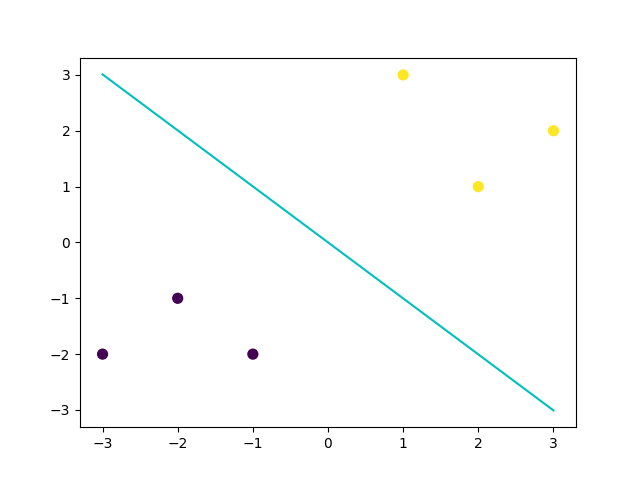
# 可视化决策边界
plt.figure()
plt.scatter(x_fearures[:,0],x_fearures[:,1], c=y_label, s=50, cmap='viridis')
plt.plot(x_range, y_3, '-c')
plt.show()

the weight of Logistic Regression: [[0.33364706 0.33270588]]
the intercept(w0) of Logistic Regression: [-0.00031373]
The prediction result: [0 0 0 1 1 1]