Visium HD使用Cellpose进行细胞分割获取单细胞精度空间数据

本文链接：https://blog.csdn.net/bio_multiomics/article/details/144752451

Visium HD为了获取单细胞级数据，前面我们介绍了基于高清的H&E图像使用StarDist进行细胞核分割，然后将覆盖在识别出来的细胞核区域上的2um bin进行合并，将这些合并的bins当做一个细胞进行后续分析。

不管是10x官方提供的细胞核分割方法(https://www.10xgenomics.com/analysis-guides/segmentation-visium-hd), 或是bin2cell (https://github.com/Teichlab/bin2cell), 抑或是上节我们测试的ENACT (https://github.com/Sanofi-Public/enact-pipeline)其本质都是一样的，使用StarDist预训练的2D_versatile_he模型首先识别细胞核轮廓，然后将覆盖在细胞核轮廓上的bins进行合并，无非是bin-to-cell合并的方法不同罢了。

需要特别强调下，只要是使用StarDist预训练的2D_versatile_he模型进行分割的，那一定分割的是细胞核，尽管StarDist也是可以进行细胞轮廓识别，但是2D_versatile_he模型是使用DAPI染的细胞核图像训练的，而上面我们说的3种分割都是用的2D_versatile_he模型，所以记住它们都是细胞和分割，分割后bin-to-cell获取的是接近snRNA-seq结果会丢失细胞质的表达信息。

为了识别出细胞边界，我们可以使用Cellpose (https://www.cellpose.org/)进行单细胞分割，然后再bin-to-cell获得的就是单细胞精度的数据了。

Cellpose提供了多种预训练模型，主要包括2类：

1. 细胞质模型（cyto）：适用于细胞质分割，通常用于处理细胞形态较为复杂的图像。

2. 细胞核模型（nuclei）：专门用于细胞核的分割，适合于需要高精度核定位的应用。

Cellpose在Visium HD数据细胞分割中的优势：

高分辨率细胞分割：

Cellpose作为一种深度学习模型，能够有效地处理这些高分辨率图像，提供精确的细胞分割，从而确保后续分析的准确性；

自动化处理：

Cellpose能够自动识别和分割图像中的细胞，减少了人工标注的需求；

适应性强：

Cellpose经过多样化的数据集训练，具有较强的通用性，能够适应不同类型的细胞图像，而无需用户进行大量的重新训练或调整参数；

支持复杂组织结构：

Cellpose能够有效处理复杂且细胞密度较高且复杂的组织结构，能准确识别重叠细胞和多样化形态，提高分割精度。

以下是使用Cellpose进行细胞分割，然后将2um bin基因表达合并得到单细胞精度表达数据，代码我都进行了详细注释。

# 导入必要的库
import numpy as np
import pandas as pd
import scanpy as sc
import tifffile
import geopandas as gpd
from shapely.geometry import Point
from cellpose import models, core

# 定义读取图像的函数，并可选择下采样因子
def read_dapi_image(img_path: str, downscale_factor: int = 2) -> np.ndarray:
    img = io.imread(img_path)  # 读取图像文件
    print(img.shape)  # 打印图像的形状
    return downscale_image(img, downscale_factor=downscale_factor)  # 返回下采样后的图像

# 定义下采样图像的函数
def downscale_image(img: np.ndarray, downscale_factor: int = 2) -> np.ndarray:
    # 计算每个轴上所需的填充量
    pad_height = (downscale_factor - img.shape[0] % downscale_factor) % downscale_factor
    pad_width = (downscale_factor - img.shape[1] % downscale_factor) % downscale_factor
    new_shape = (img.shape[0] + pad_height, img.shape[1] + pad_width, img.shape[2])  # 新图像形状
    new_image = np.zeros(new_shape, dtype=img.dtype)  # 创建新的零填充图像
    for channel in range(img.shape[2]):
        new_image[:, :, channel] = np.pad(
            img[:, :, channel], ((0, pad_height), (0, pad_width)), mode="constant"
        )  # 对每个通道进行零填充
    return new_image  # 返回填充后的图像

# 定义运行Cellpose进行细胞分割的函数
def run_cellpose(img: np.ndarray, model_path: str):
    use_GPU = core.use_gpu()  # 检查是否使用GPU
    model = models.CellposeModel(gpu=use_GPU, pretrained_model=model_path)  # 加载Cellpose模型
    channels = [0, 0]  # 设置通道（这里假设为单通道）
    masks, flows, styles = model.eval(
        [img],
        channels=channels,
        diameter=model.diam_labels,
        flow_threshold=1,
        cellprob_threshold=0,
        batch_size=4,
    )  # 执行细胞分割并返回掩膜、流和样式信息
    return (masks, flows, styles)  # 返回分割结果

# 设置Visium HD数据的文件路径并读取图像
img_path = "./data/visiumHD_colorectal_cancer/P1_CRC/Visium_HD_Human_Colon_Cancer_P1_tissue_image.btf"
maxed_visium = read_dapi_image(img_path, downscale_factor=1)  # 读取并下采样图像

# 设置分块参数和模型路径
chunk_per_axis = 2  # 每个轴上分块数目
mp = 'cyto'  # 使用细胞质模型进行分割

# 对图像进行分块并调用Cellpose进行细胞分割
masks_top_left, flows, styles = run_cellpose(
    maxed_visium[
        : np.shape(maxed_visium)[0] // chunk_per_axis,
        : np.shape(maxed_visium)[1] // chunk_per_axis,
        :,
    ],
    model_path=mp,
)
masks_top_right, flows, styles = run_cellpose(
    maxed_visium[
        : np.shape(maxed_visium)[0] // chunk_per_axis,
        np.shape(maxed_visium)[1] // chunk_per_axis :,
        :,
    ],
    model_path=mp,
)
masks_bottom_left, flows, styles = run_cellpose(
    maxed_visium[
        np.shape(maxed_visium)[0] // chunk_per_axis :,
        : np.shape(maxed_visium)[1] // chunk_per_axis,
        :,
    ],
    model_path=mp,
)
masks_bottom_right, flows, styles = run_cellpose(
    maxed_visium[
        np.shape(maxed_visium)[0] // chunk_per_axis :,
        np.shape(maxed_visium)[1] // chunk_per_axis :,
        :,
    ],
    model_path=mp,
)

# 初始化全掩膜数组，准备合并分块结果
constant = 1000000  # 用于区分不同块的常量值
full_mask = np.zeros_like(maxed_visium[:, :, 0], dtype=np.uint32)  # 创建与原图相同大小的掩膜数组

# 将各个块的掩膜合并到全掩膜中，并加上常量以区分不同区域
full_mask[
    : np.shape(maxed_visium)[0] // chunk_per_axis,
    : np.shape(maxed_visium)[1] // chunk_per_axis,
] = masks_top_left[0]
full_mask[
    : np.shape(maxed_visium)[0] // chunk_per_axis,
    np.shape(maxed_visium)[1] // chunk_per_axis :,
] = masks_top_right[0] + (constant)
full_mask[
    np.shape(maxed_visium)[0] // chunk_per_axis :,
    : np.shape(maxed_visium)[1] // chunk_per_axis,
] = masks_bottom_left[0] + (constant * 2)
full_mask[
    np.shape(maxed_visium)[0] // chunk_per_axis :,
    np.shape(maxed_visium)[1] // chunk_per_axis :,
] = masks_bottom_right[0] + (constant * 3)

# 将全掩膜中值为常量的部分设置为0，表示没有细胞
full_mask = np.where(full_mask % constant == 0, 0, full_mask)

# 将全掩膜保存为PNG格式文件
tifffile.imsave("./visium_hd/segmentation.png", full_mask)
# 设置Visium HD数据目录路径以加载空间转录组数据
dir_base = "./data/visiumHD_colorectal_cancer/P1_CRC/outs/binned_outputs/square_002um/"

# 加载Visium HD数据中的基因表达矩阵（HDF5格式）
raw_h5_file = dir_base + "filtered_feature_bc_matrix.h5"
adata = sc.read_10x_h5(raw_h5_file)  # 使用Scanpy读取数据

# 加载组织位置坐标文件（Parquet格式）
tissue_position_file = dir_base + "spatial/tissue_positions.parquet"
df_tissue_positions = pd.read_parquet(tissue_position_file)

# 将数据框的索引设置为条形码，以便后续合并操作使用
df_tissue_positions = df_tissue_positions.set_index("barcode")

# 在数据框中创建索引以检查合并情况
df_tissue_positions["index"] = df_tissue_positions.index

# 将组织位置添加到AnnData对象的元数据中（obs）
adata.obs = pd.merge(adata.obs, df_tissue_positions, left_index=True, right_index=True)

# 从坐标数据框创建GeoDataFrame，以便进行空间分析
geometry = [
    Point(xy)
    for xy in zip(
        df_tissue_positions["pxl_col_in_fullres"],
        df_tissue_positions["pxl_row_in_fullres"],
    )
]
gdf_coordinates = gpd.GeoDataFrame(df_tissue_positions, geometry=geometry)

## 将捕获区域分配给单个细胞
# 检查点掩膜是否在全掩膜范围内，以确保坐标有效性
point_mask = (
    gdf_coordinates["pxl_row_in_fullres"].values.astype(int) < np.shape(full_mask)[0]
) & (gdf_coordinates["pxl_col_in_fullres"].values.astype(int) < np.shape(full_mask)[1])

# 根据有效坐标从全掩膜中提取细胞ID信息
cells = full_mask[
    gdf_coordinates["pxl_row_in_fullres"].values.astype(int)[point_mask],
    gdf_coordinates["pxl_col_in_fullres"].values.astype(int)[point_mask],
]
gdf_coordinates = gdf_coordinates[point_mask]
gdf_coordinates["cells"] = cells  # 将细胞ID添加到GeoDataFrame中
assigned_regions = gdf_coordinates[gdf_coordinates["cells"] > 0]

# 将细胞ID信息合并到AnnData对象中，以便后续分析使用
adata.obs = adata.obs.merge(
    assigned_regions[["cells"]], left_index=True, right_index=True, how="left"
)
adata = adata[~pd.isna(adata.obs["cells"])]  # 移除没有细胞ID的数据行
adata.obs["cells"] = adata.obs["cells"].astype(int)  # 将细胞ID转换为整数类型

## 在捕获区域内汇总转录本计数
from scipy import sparse

# 按唯一细胞ID对数据进行分组，以便汇总转录本计数
groupby_object = adata.obs.groupby(["cells"], observed=True)
counts = adata.X  # 提取基因表达计数矩阵
spatial_coords = adata.obs[["pxl_row_in_fullres", "pxl_col_in_fullres"]].values
N_groups = groupby_object.ngroups  # 获取唯一细胞ID数量（组数）
N_genes = counts.shape[1]  # 获取基因数量

# 初始化稀疏矩阵以存储每个细胞的基因计数汇总结果
summed_counts = sparse.lil_matrix((N_groups, N_genes))
polygon_id = []  # 存储多边形ID列表
cell_coords = []  # 存储细胞坐标列表
row = 0

# 遍历每个唯一多边形，计算基因计数的总和。
for polygons, idx_ in groupby_object.indices.items():
    summed_counts[row] = counts[idx_].sum(0)  # 汇总该多边形内所有细胞的基因计数
    cell_coords.append(np.mean(spatial_coords[idx_], axis=0))  # 获取该多边形内细胞坐标均值作为代表坐标
    row += 1
    polygon_id.append(polygons)  # 添加多边形ID到列表中
cell_coords = np.array(cell_coords)  
summed_counts = summed_counts.tocsr()  # 转换为压缩稀疏行矩阵格式

# 创建一个新的AnnData对象，用于存储汇总后的基因计数矩阵及其元数据。
grouped_adata = anndata.AnnData(
    X=summed_counts,
    obs=pd.DataFrame(polygon_id, columns=["cells"], index=polygon_id),
    var=adata.var,
)
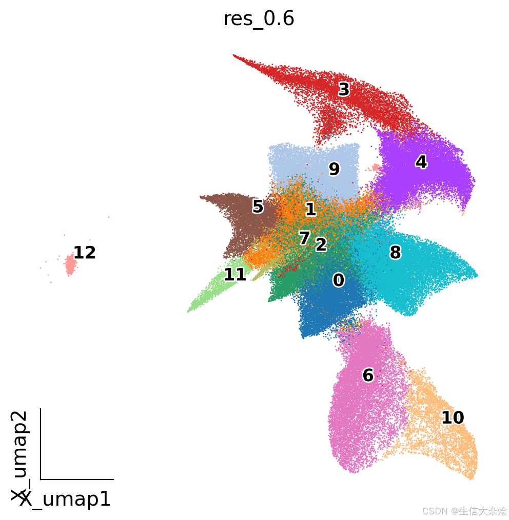
grouped_adata.write('adata_cellpose.h5ad')

拿到细胞分割后的结果后，降维聚类看下结果，对比之前合并8um bin结果看起来，大群基本上分开了，效果挺好。

题外话

其实我们还可以使用Qupath导入H&E图像，使用Cellpose或者一些开源的机器学习算法可视化进行细胞分割，好处是可以自己训练模型，然后细胞分割后直观就能看到，如果不满意就可以微调参数进行分割，直到能将绝大多数细胞分割出来，最后可以导出这些细胞的坐标信息，然后就是使用上面bin-to-cell部分的代码，就能达到更好的结果。

微信公众号: 生信大杂烩