【A图像分类实战】2024 Pytorch搭建AlexNet、VGG16、GoogleNet等共5个模型实现COIL20数据集图像20分类完整项目(项目已开源）

置顶北村南

已于 2024-03-07 09:18:24 修改

阅读量3.4k

点赞数 27

分类专栏：《深度学习》文章标签： pytorch 深度学习人工智能

于 2022-12-07 16:07:55 首次发布

本文链接：https://blog.csdn.net/ccaoshangfei/article/details/128185277

版权

《深度学习》专栏收录该内容

12 篇文章 82 订阅

订阅专栏

🍊本项目使用Pytorch框架，使用end-end的结构实现COIL20图像分类

🍊神经网络模型可选择LeNet、AlexNet、GoogleNet、VGG16、ResNet50、EfficientNet（Doing）

🍊项目已开源

🍊修改少了参数即可适配读者自己的数据集

🍊网络模型易扩展，可作BaseLine

🍊敲完这6个模型，相当于浅走了一遍CNN的前世今生

🍊最终准确率均达到了100%（COIL20为易数据集）

🍊结合原论文讲解(附论文地址)，并适配于COIL20数据集

一、Introduction

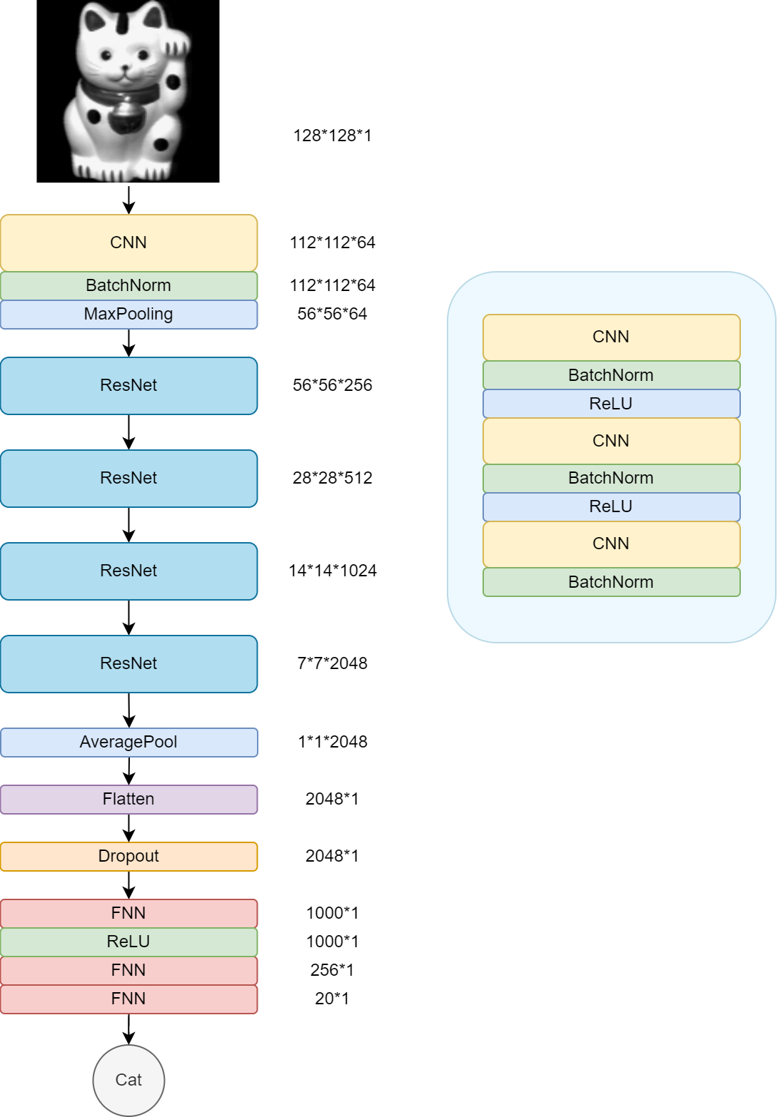
1.1 网络架构图

该网络模型主要使用上游特征提取模型+下游分类器模型组成

1.2 快速使用

该项目已开源在Github上，地址为 Coil20_Image_Classfiation

抑或使用Git下载

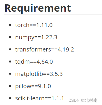
git cloen https://github.com/BeiCunNan/Coil20_Image_Classfiation.git

主要环境要求如下（环境莫过于太老基本没啥问题的）

下载该项目后，配置相对应的环境，在config.py文件中自行选择所需的神经网络模型，如下图所示，最后运行main.py文件即可

1.3 工程结构

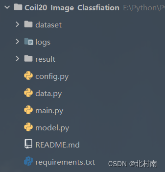
dataset：数据集
logs：训练日志
result：Loss、Acc训练过程图
config.py：配置文件
data.py：制作DataSet和DataLoader
main.py：主函数，负责全流程项目运行，包括模型的训练和测试
model.py：神经网络模型

1.4 基础知识

如果有小伙伴还不是很懂CNN、Kernal、Stride、Pooling的话，建议先看以下篇文章

【Deep Learning】CNN卷积神经网络

二、Config

作者看了很多论文源代码中都使用parser容器进行全局变量的配置，因此也照葫芦画瓢编写了config.py文件

import os
import sys
import time
import torch
import random
import logging
import argparse
from datetime import datetime


def get_config():
    parser = argparse.ArgumentParser()

    '''Base'''
    parser.add_argument('--num_classes', type=int, default=20)
    parser.add_argument('--model_name', type=str, default='VGG16',
                        choices=['LeNet', 'AlexNet', 'GoogleNet', 'VGG16', 'ResNet50', 'EfficientNet'])

    '''Optimization'''
    parser.add_argument('--train_batch_size', type=int, default=32)
    parser.add_argument('--test_batch_size', type=int, default=32)
    parser.add_argument('--num_epoch', type=int, default=10)
    parser.add_argument('--lr', type=float, default=1e-4)
    parser.add_argument('--weight_decay', type=float, default=0.01)

    '''Environment'''
    parser.add_argument('--device', type=str, default='cuda')
    parser.add_argument('--backend', default=False, action='store_true')
    parser.add_argument('--workers', type=int, default=0)
    parser.add_argument('--timestamp', type=int, default='{:.0f}{:03}'.format(time.time(), random.randint(0, 999)))
    parser.add_argument('--index', type=int, default=0)

    args = parser.parse_args()
    args.device = torch.device(args.device)

    '''logger'''
    args.log_name = '{}_{}.log'.format(args.model_name, datetime.now().strftime('%Y-%m-%d_%H-%M-%S')[2:])
    if not os.path.exists('logs'):
        os.mkdir('logs')
    logger = logging.getLogger()
    logger.setLevel(logging.INFO)
    logger.addHandler(logging.StreamHandler(sys.stdout))
    logger.addHandler(logging.FileHandler(os.path.join('logs', args.log_name)))
    return args, logger

三、Data

3.1 数据准备

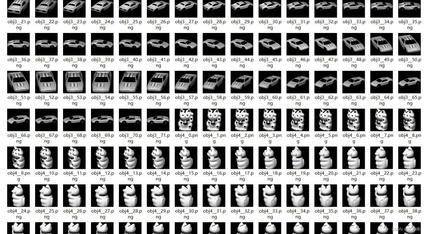
COIL20数据集一共有20种对象，每个对象均有72个样本，因此一共有1440个样本，我们按照9:1来划分训练集和测试集，这里展示部分数据

3.2 制作DataSet

代码细节：使用glob函数来获取所有图片的路径

    all_imgs_path = glob.glob(r'dataset\*.png')
    for ip in all_imgs_path:
        data.append(ip)

代码细节：随后使用PIL的Image函数来打开图片，并将其转换成Tensor，最后组合成(图片，标签)来存储到DataSet中

class Mydataset(Dataset):
    def __init__(self, images, labels, transform):
        self.images = images
        self.labels = labels
        self.transform = transform
        dataset = []
        for i in range(len(labels)):
            temp_img = Image.open(images[i])
            temp_img = self.transform(temp_img)
            dataset.append((temp_img, labels[i]))
        self.dataset = dataset

    def __getitem__(self, index):
        return self.dataset[index]

    def __len__(self):
        return len(self.labels)

值得注意的是，这里图片初始化尺寸是可以调整的，因此你可以在此修改来适配您自己的数据集，比如自己的数据集为64*64，就改为transformers.Resieze((64,64))

    transform = transforms.Compose([
        transforms.Resize((128, 128)),
        transforms.ToTensor()
    ])

3.3 制作DataLoader

    tr_loader = DataLoader(tr_set, batch_size=self.args.train_batch_size, shuffle=True, num_workers=self.args.workers,
                           pin_memory=True)
    te_loader = DataLoader(te_set, batch_size=self.args.train_batch_size, shuffle=True, num_workers=self.args.workers,
                           pin_memory=True)

四、Model

4.1 Overview

让我们先看看CNN的发展历史，以下的模型讲解也是按照发展历史来

模型	时间	贡献
LeNet	1998	CNN 开山之作 Sigmoid 激活函数
AlexNet	2012	ReLu 激活函数 Dropout 防过拟合 MaxPool 最大池化
GoogLeNet	2014	平行架构，增模型宽度 1*1 卷积核
VGG16	2014	只用3*3小卷积 Padding保持图像大小不变，深度增加
ResNet	2018	残差解决退化问题
EfficientNet	2020	组合缩放快而准

4.2 CNN calculation formula

在看网络模型之前，还是值得提一提CNN中卷积的计算公式，如此可更好理解后面的网络模型

N：输出图片边长
W：输入图片边长
F：kernel大小
S：stride步长
P：padding补缺数量

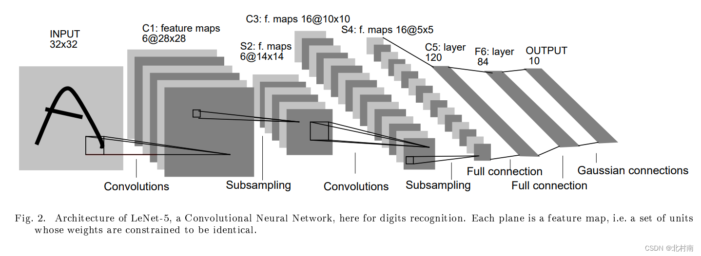
4.3 LeNet 1998

论文地址《Gradient-Based Learning Applied to Document Recognition》

原始网络结构

使用CNN+Sigmoid串行组合来进行特征提取，最后使用Flatten+FNN进行分类预测

适配网络结构

根据自己图像尺寸修改第一个CNN
加入了Dropout层使模型的鲁棒性更好

代码

class LeNet(torch.nn.Module):
    def __init__(self):
        super(LeNet, self).__init__()
        self.convs = nn.Sequential(
            nn.Conv2d(1, 10, 10, 2),
            nn.Sigmoid(),
            nn.MaxPool2d(2, 2),

            nn.Conv2d(10, 20, 5),
            nn.Sigmoid(),
            nn.MaxPool2d(2, 2),

            nn.Conv2d(20, 20, 4),
            nn.Sigmoid(),
            nn.MaxPool2d(2, 2),

            nn.Conv2d(20, 20, 3, 1, 1),
            nn.Sigmoid(),
        )

        self.fc = nn.Sequential(
            nn.Dropout(0.5),
            nn.Linear(5 * 5 * 20, 100),
            nn.Sigmoid(),
            nn.Linear(100, 60),
            nn.Sigmoid(),
            nn.Linear(60, 20)
        )

    def forward(self, x):
        batch_size = x.size(0)
        x = self.convs(x)
        x = x.view(batch_size, -1)
        x = self.fc(x)
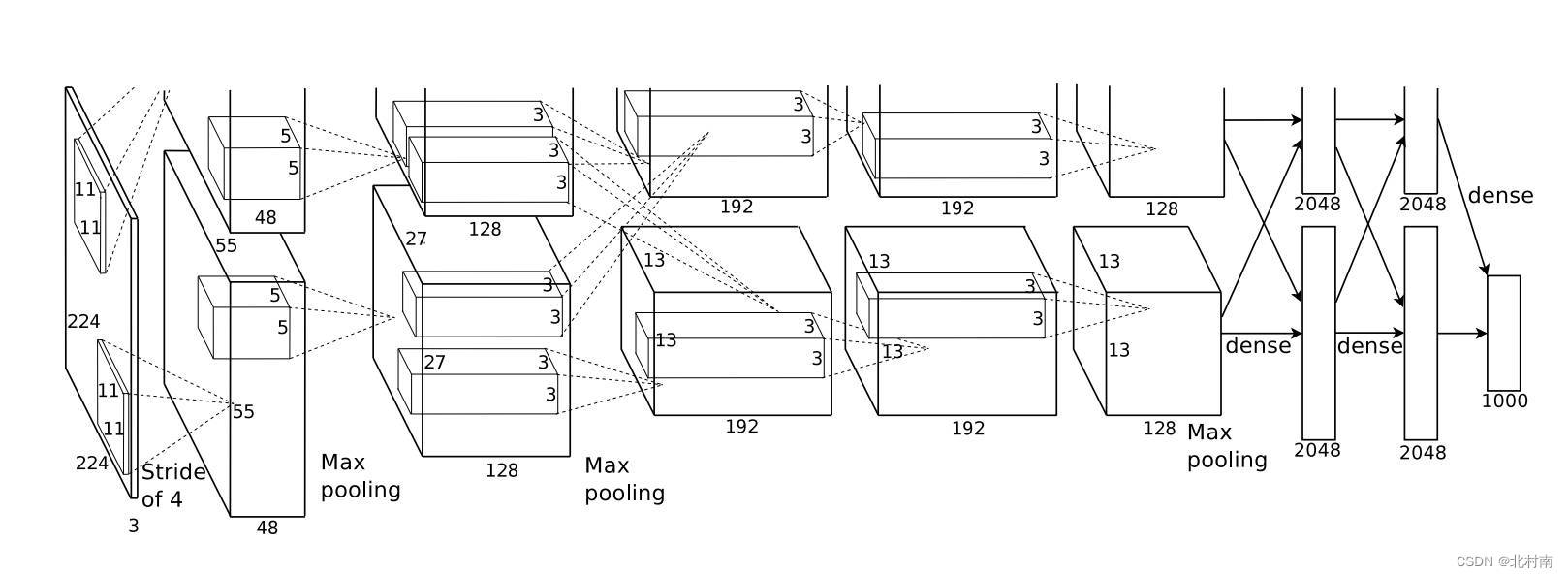
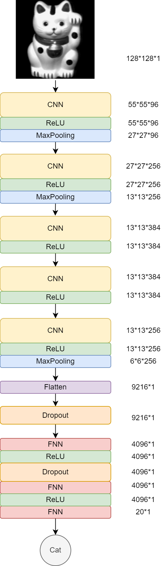
        return x

4.4 AlexNet 2012

论文地址《ImageNet Classifification with Deep Convolutional Neural Networks》

原始网络结构

使用CNN+ReLu串行组合来进行特征提取，最后使用Dropout+Flatten+FNN进行分类预测

适配网络结构

根据自己图像尺寸修改第一个CNN
双层模型改为单层模型

代码

class AlexNet(torch.nn.Module):
    def __init__(self):
        super(AlexNet, self).__init__()
        self.convs = nn.Sequential(
            nn.Conv2d(in_channels=1, out_channels=96, kernel_size=20, stride=2),
            nn.ReLU(inplace=True),
            nn.MaxPool2d(kernel_size=3, stride=2),

            nn.Conv2d(in_channels=96, out_channels=256, kernel_size=5, stride=1, padding=2),
            nn.ReLU(inplace=True),
            nn.MaxPool2d(kernel_size=3, stride=2),

            nn.Conv2d(in_channels=256, out_channels=384, kernel_size=3, stride=1, padding=1),
            nn.ReLU(inplace=True),

            nn.Conv2d(in_channels=384, out_channels=384, kernel_size=3, stride=1, padding=1),
            nn.ReLU(inplace=True),

            nn.Conv2d(in_channels=384, out_channels=256, kernel_size=3, stride=1, padding=1),
            nn.ReLU(inplace=True),
            nn.MaxPool2d(kernel_size=3, stride=2)
        )
        self.fc = nn.Sequential(
            nn.Dropout(0.5),
            nn.Linear(in_features=256 * 6 * 6, out_features=4096),
            nn.ReLU(inplace=True),
            nn.Dropout(0.5),
            nn.Linear(in_features=4096, out_features=4096),
            nn.ReLU(inplace=True),
            nn.Linear(in_features=4096, out_features=20)
        )

    def forward(self, x):
        batch_size = x.size(0)
        x = self.convs(x)
        x = x.view(batch_size, -1)
        x = self.fc(x)
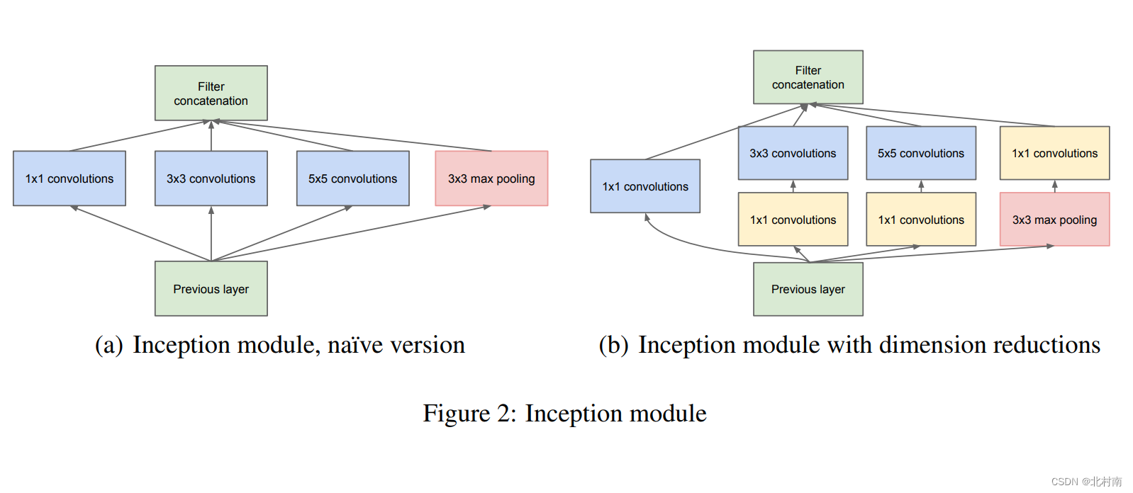
        return x

4.5 GoogLeNet 2014

论文地址《Going deeper with convolutions》

原始网络结构

GoogLeNet主要是由9个称之为Inception的模块堆叠而成，每个Inception的模块如下图(b)所示，即从一个Layer中分出4个小CNN模块，最后将4个小CNN模块进行拼接组合。

关于为什么要怎么做，作者的理解是其实在CNN中一直有个困扰大家的问题，即Kernal的尺寸和深度到底要怎么选？粗鲁的做法是，如果不知道怎么选那我们将所有的可能性都先列出来，即下方的1*1、3*3、5*5的Kernal，然后使用类似机器学习中的Soft-Voting做法来给每个小CNN模块一个权重。

除此之外，这个做法和2018年RestNet的做法又有异曲同工之妙，ResNet在下面4.7中会介绍，读者可先看完GoogLeNet和ResNet网络之后再思考此问题。

为什么说异曲同工之妙呢，因此残差机制的直观理解就是可以恒等映射，跳过几个效果不好的CNN来提高深度，在这里，我们使用了1*1的Kernal，其实也可以认为是恒等映射，我们极端的讲好了，如果3*3、5*5的卷积效果都不好，那网络都给他们权重都是0好了，那自然这4个小CNN模块只有1*1的CNN模块有效了,若这个1*1的CNN权重参数均为1，那就是完全的恒等映射了。

除此之外，GoogLeNet的最终的分类预测也很有意思，它没有使用传统的Flatten，而是使用AveragePooling，据原论文报道使用该方法后模型的Acc可以提高1个点左右，当然最后还是使用了一个FNN，这是为了便于下游任务的Fine Tuning

其网络模块的参数如下

适配网络结构

根据自己图像尺寸修改第一个CNN

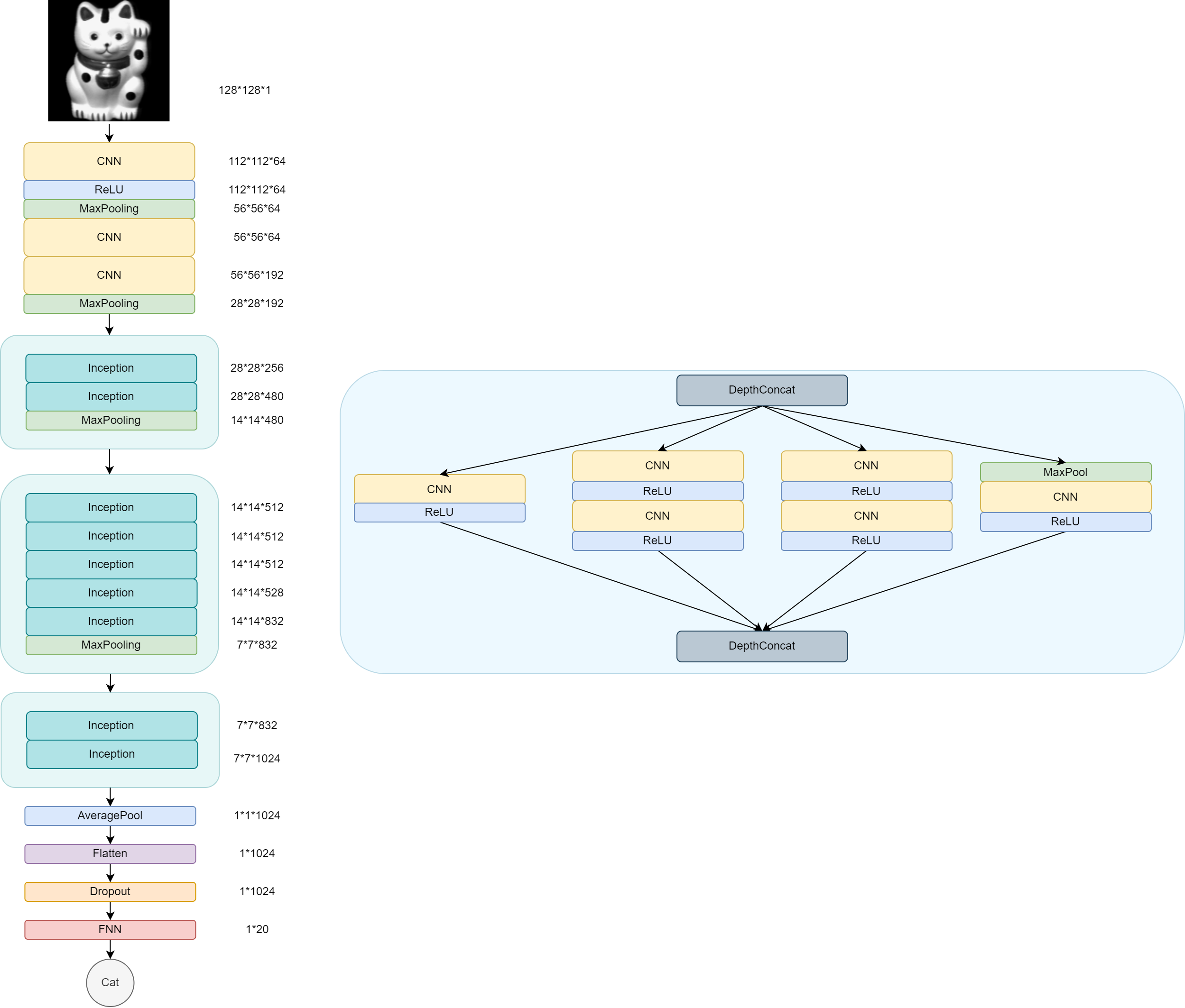
代码

每个CNN都加上一个ReLU激活函数

class BasicConv2d(nn.Module):
    def __init__(self, in_channels, out_channels, **kwargs):
        super(BasicConv2d, self).__init__()
        self.conv = nn.Conv2d(in_channels, out_channels, **kwargs)
        self.relu = nn.ReLU(inplace=True)

    def forward(self, x):
        x = self.conv(x)
        x = self.relu(x)
        return x

Inception模块

class Inception(nn.Module):
    def __init__(self, in_channels, ch1x1, ch3x3red, ch3x3, ch5x5red, ch5x5, pool_proj):
        super(Inception, self).__init__()

        self.branch1 = BasicConv2d(in_channels, ch1x1, kernel_size=1)

        self.branch2 = nn.Sequential(
            BasicConv2d(in_channels, ch3x3red, kernel_size=1),
            BasicConv2d(ch3x3red, ch3x3, kernel_size=3, padding=1)
        )

        self.branch3 = nn.Sequential(
            BasicConv2d(in_channels, ch5x5red, kernel_size=1),
            BasicConv2d(ch5x5red, ch5x5, kernel_size=5, padding=2)
        )

        self.branch4 = nn.Sequential(
            nn.MaxPool2d(kernel_size=3, stride=1, padding=1),
            BasicConv2d(in_channels, pool_proj, kernel_size=1)
        )

    def forward(self, x):
        branch1 = self.branch1(x)
        branch2 = self.branch2(x)
        branch3 = self.branch3(x)
        branch4 = self.branch4(x)

        outputs = [branch1, branch2, branch3, branch4]
        return torch.cat(outputs, 1)

主体模型

class GoogleNet(nn.Module):
    def __init__(self):
        super(GoogleNet, self).__init__()
        self.inputs = nn.Sequential(nn.Conv2d(in_channels=1, out_channels=64, kernel_size=17),
                                    nn.ReLU(),
                                    nn.MaxPool2d(kernel_size=3, stride=2, padding=1),
                                    nn.Conv2d(64, 64, kernel_size=1),
                                    nn.Conv2d(64, 192, kernel_size=3, padding=1),
                                    nn.MaxPool2d(kernel_size=3, stride=2, padding=1))
        self.block1 = nn.Sequential(
            Inception(192, 64, 96, 128, 16, 32, 32),
            Inception(256, 128, 128, 192, 32, 96, 64),
            nn.MaxPool2d(kernel_size=3, stride=2, padding=1)
        )
        self.block2 = nn.Sequential(Inception(480, 192, 96, 208, 16, 48, 64),
                                    Inception(512, 160, 112, 224, 24, 64, 64),
                                    Inception(512, 128, 128, 256, 24, 64, 64),
                                    Inception(512, 112, 144, 288, 32, 64, 64),
                                    Inception(528, 256, 160, 320, 32, 128, 128),
                                    nn.MaxPool2d(kernel_size=3, stride=2, padding=1)
                                    )
        self.block3 = nn.Sequential(
            Inception(832, 256, 160, 320, 32, 128, 128),
            Inception(832, 384, 192, 384, 48, 128, 128),
        )
        self.avgpool = nn.AdaptiveAvgPool2d((1, 1))
        self.outputs = nn.Sequential(
            nn.Dropout(0.5),
            nn.Linear(1024, 20)
        )

    def forward(self, x):
        batch_size = x.size(0)
        x = self.inputs(x)
        x = self.block1(x)
        x = self.block2(x)
        x = self.block3(x)
        x = self.avgpool(x)
        x = x.view(batch_size, -1)
        x = self.outputs(x)
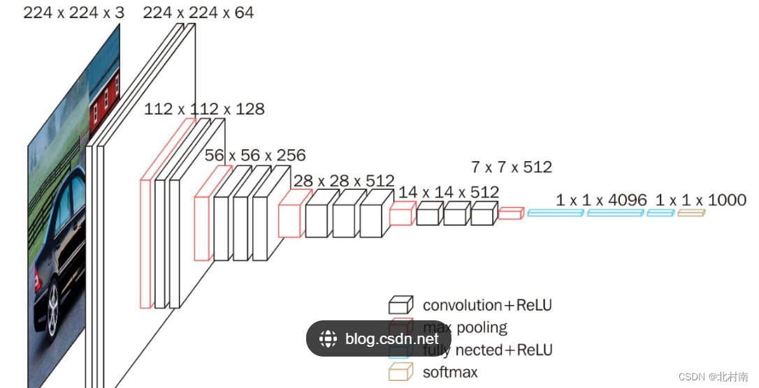
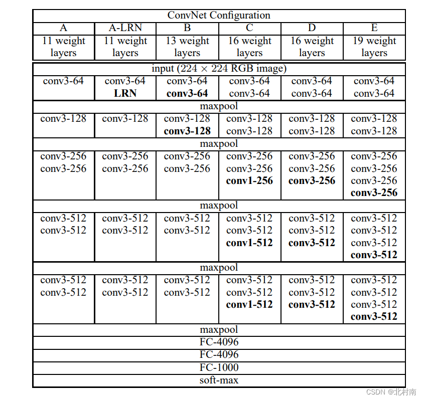
        return x

4.6 VGG16 2014

论文地址《Very deep convolutional networks for large-scaleimage recognition》

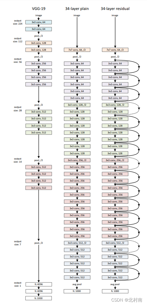
原始网络结构

只使用最简单的3*3的Kernal和Pool进行串行组合，同时使用Padding技术使得图像经过Kernal大小保持不变，从而可以在保持图像大小不变的情况下深度挖掘图像中的信息

适配网络结构

根据自己图像尺寸修改第一个CNN

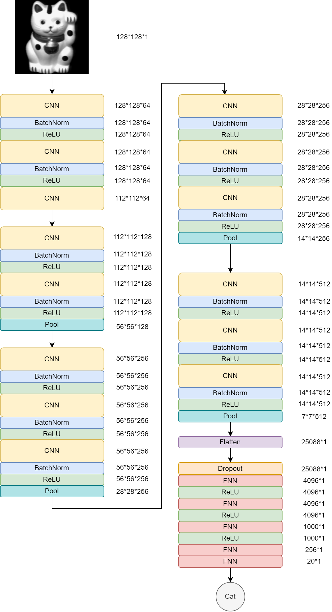
在代码部分我们放入了BatchNorm进行Batch归一化处理，这使得数据在进行Relu之前不会因为数据过大而导致网络性能的不稳定，BatchNorm2d()函数数学原理如下：

代码

class VGG16(torch.nn.Module):
    def __init__(self):
        super(VGG16, self).__init__()
        self.block1 = nn.Sequential(
            nn.Conv2d(in_channels=1, out_channels=64, kernel_size=3, stride=1, padding=1),
            nn.BatchNorm2d(64),
            nn.ReLU(inplace=True),

            nn.Conv2d(in_channels=64, out_channels=64, kernel_size=3, stride=1, padding=1),
            nn.BatchNorm2d(64),
            nn.ReLU(inplace=True),

            nn.Conv2d(in_channels=64, out_channels=64, kernel_size=17)
        )
        self.block2 = nn.Sequential(
            nn.Conv2d(in_channels=64, out_channels=128, kernel_size=3, stride=1, padding=1),
            nn.BatchNorm2d(128),
            nn.ReLU(inplace=True),
            nn.Conv2d(in_channels=128, out_channels=128, kernel_size=3, stride=1, padding=1),
            nn.BatchNorm2d(128),
            nn.ReLU(inplace=True),

            nn.MaxPool2d(2, 2)
        )
        self.block3 = nn.Sequential(
            nn.Conv2d(in_channels=128, out_channels=256, kernel_size=3, stride=1, padding=1),
            nn.BatchNorm2d(256),
            nn.ReLU(inplace=True),
            nn.Conv2d(in_channels=256, out_channels=256, kernel_size=3, stride=1, padding=1),
            nn.BatchNorm2d(256),
            nn.ReLU(inplace=True),
            nn.Conv2d(in_channels=256, out_channels=256, kernel_size=3, stride=1, padding=1),          
            nn.BatchNorm2d(256),
            nn.ReLU(inplace=True),
            nn.MaxPool2d(2, 2)
        )
        self.block4 = nn.Sequential(
            nn.Conv2d(in_channels=256, out_channels=512, kernel_size=3, stride=1, padding=1),
            nn.BatchNorm2d(512),
            nn.ReLU(inplace=True),
            nn.Conv2d(in_channels=512, out_channels=512, kernel_size=3, stride=1, padding=1),
            nn.BatchNorm2d(512),
            nn.ReLU(inplace=True),
            nn.Conv2d(in_channels=512, out_channels=512, kernel_size=3, stride=1, padding=1),
            nn.BatchNorm2d(512),
            nn.ReLU(inplace=True),
            nn.MaxPool2d(2, 2)
        )
        self.block5 = nn.Sequential(
            nn.Conv2d(in_channels=512, out_channels=512, kernel_size=3, stride=1, padding=1),
            nn.BatchNorm2d(512),
            nn.ReLU(inplace=True),
            nn.Conv2d(in_channels=512, out_channels=512, kernel_size=3, stride=1, padding=1),
            nn.BatchNorm2d(512),
            nn.ReLU(inplace=True),
            nn.Conv2d(in_channels=512, out_channels=512, kernel_size=3, stride=1, padding=1),
            nn.BatchNorm2d(512),
            nn.ReLU(inplace=True),
            nn.MaxPool2d(2, 2)
        )
        self.convs = nn.Sequential(
            self.block1,
            self.block2,
            self.block3,
            self.block4,
            self.block5
        )
        self.fnn = nn.Sequential(
            nn.Dropout(0.5),
            nn.Linear(25088, 4096),
            nn.ReLU(inplace=True),
            nn.Linear(4096, 4096),
            nn.ReLU(inplace=True),
            nn.Linear(4096, 1000),
            nn.ReLU(inplace=True),
            nn.Linear(1000, 256),
            nn.Linear(256, 20),
        )

    def forward(self, x):
        batch_size = x.size(0)
        x = self.convs(x),
        x = x[0]
        x = x.view(batch_size, -1)
        x = self.fnn(x)
        return x

4.7 ResNet 2018

论文地址《Deep Residual Learning for Image Recognition》

原始网络结构

原始论文中的两层残差块叫做Shortcut connection，用于最原始的ResNet18和ResNet34

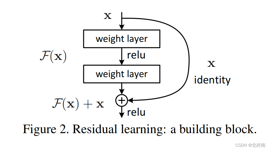
而这里我们使用的是Rest50，其残差块有三层，称之为Bottleneck，中间一层为3*3的Kernal，而两侧是1*1的Kernal，1*1的Kernal主要是用来改变channels大小（在RestNet中是将channels乘4）

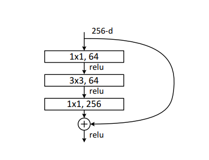
几个Bottleneck组合成一个Block，在ReNet50中一共有4个Block，各个Block含有的Bottleneck的数量分别为3,4,3,6

在每个Block的第一个Bottleneck的输入和输出会组合成Shortcut connection，即残差就是体现在这里

适配网络结构

根据自己图像尺寸修改第一个CNN

代码

残差块设计

class Bottleneck(nn.Module):
    def __init__(self, in_channels, out_channels, stride=None, padding=None, first=False):
        super(Bottleneck, self).__init__()
        if stride is None:
            stride = [1, 1, 1]
        if padding is None:
            padding = [0, 1, 0]
        self.bottleneck = nn.Sequential(
            nn.Conv2d(in_channels, out_channels, kernel_size=1, stride=stride[0], padding=padding[0], ),
            nn.BatchNorm2d(out_channels),
            nn.ReLU(inplace=True),
            nn.Conv2d(out_channels, out_channels, kernel_size=3, stride=stride[1], padding=padding[1]),
            nn.BatchNorm2d(out_channels),
            nn.ReLU(inplace=True),
            nn.Conv2d(out_channels, out_channels * 4, kernel_size=1, stride=stride[2], padding=padding[2]),
            nn.BatchNorm2d(out_channels * 4)
        )

        if (first):
            self.res = nn.Sequential(
                nn.Conv2d(in_channels, out_channels * 4, kernel_size=1, stride=stride[1]),
                nn.BatchNorm2d(out_channels * 4)
            )
        else:
            self.res = nn.Sequential()

    def forward(self, x):
        out = self.bottleneck(x)
        out += self.res(x)
        out = F.relu(out)
        return out

总体结构

class ResNet50(nn.Module):
    def __init__(self):
        super(ResNet50, self).__init__()
        self.in_channels = 64
        self.avgpool = nn.AdaptiveAvgPool2d((1, 1))

        self.conv1 = nn.Sequential(
            nn.Conv2d(1, 64, kernel_size=17),
            nn.BatchNorm2d(64),
            nn.MaxPool2d(kernel_size=3, stride=2, padding=1)
        ) # --> 3,4,3,6
        self.conv2 = self._make_layer(Bottleneck, [[1, 1, 1]] * 3, [[0, 1, 0]] * 3, 64)
        self.conv3 = self._make_layer(Bottleneck, [[1, 2, 1]] + [[1, 1, 1]] * 3, [[0, 1, 0]] * 4, 128)
        self.conv4 = self._make_layer(Bottleneck, [[1, 2, 1]] + [[1, 1, 1]] * 5, [[0, 1, 0]] * 6, 256)
        self.conv5 = self._make_layer(Bottleneck, [[1, 2, 1]] + [[1, 1, 1]] * 2, [[0, 1, 0]] * 3, 512)

        self.convs = nn.Sequential(
            self.conv1,
            self.conv2,
            self.conv3,
            self.conv4,
            self.conv5
        )

        self.fnn = nn.Sequential(
            nn.Dropout(0.5),
            nn.Linear(2048, 1000),
            nn.ReLU(inplace=True),
            nn.Linear(1000, 256),
            nn.Linear(256, 20),
        )

    def _make_layer(self, Bottleneck, strides, paddings, out_channels):
        layers = []
        flag = True
        for i in range(len(strides)):
            layers.append(Bottleneck(self.in_channels, out_channels, strides[i], paddings[i], first=flag))
            flag = False
            self.in_channels = out_channels * 4
        return nn.Sequential(*layers)

    def forward(self, x):
        batch_size = x.size(0)
        x = self.convs(x)
        x = self.avgpool(x)
        x = x.view(batch_size, -1)
        x = self.fnn(x)
        return x

4.8 （Doing）EfficientNet 2020

论文地址《EffificientNet: Rethinking Model Scaling for Convolutional Neural Networks》

网络架构

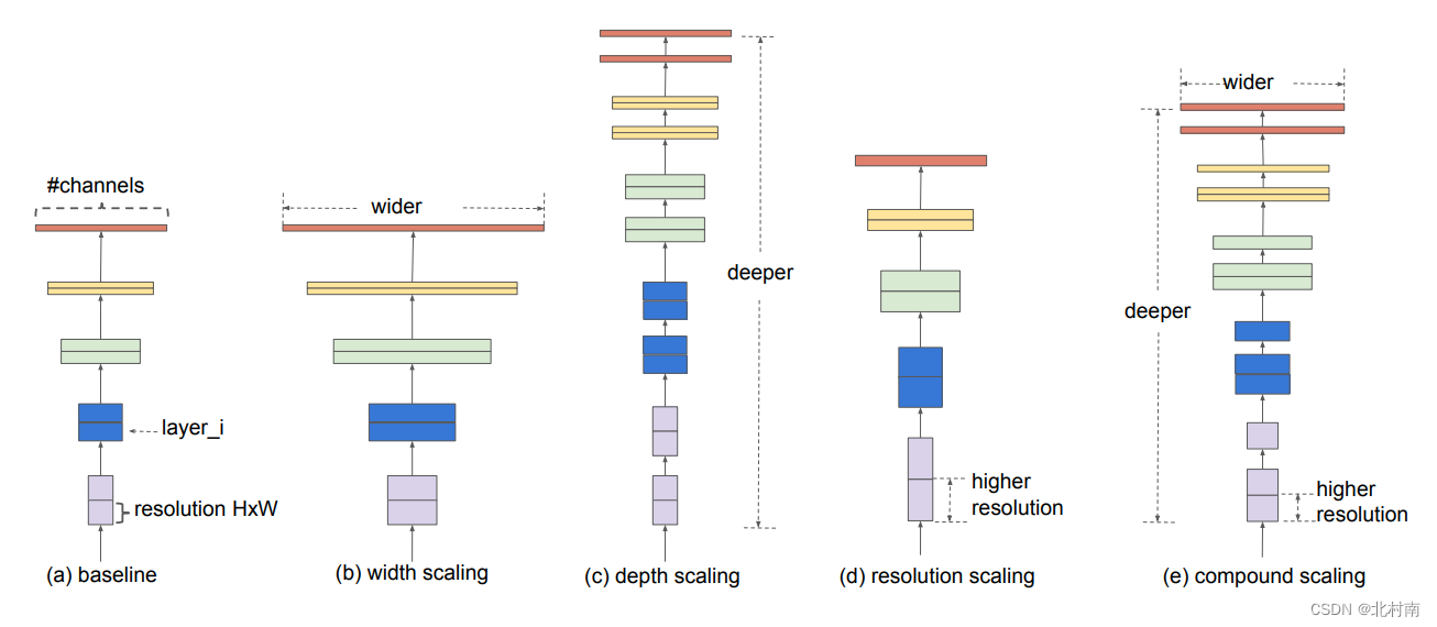
This module is being worked on。。。

五、Train and Test

训练函数

注意要开启训练模式，即self.Mymodel.train()

    def _train(self, dataloader, criterion, optimizer):
        self.args.index += 1
        train_loss, n_correct, n_train = 0, 0, 0
        # Turn on the train mode
        self.Mymodel.train()
        for inputs, targets in tqdm(dataloader, disable=self.args.backend, ascii='>='):
            inputs, targets = inputs.to(self.args.device), targets.to(self.args.device)
            predicts = self.Mymodel(inputs)
            loss = criterion(predicts, targets)

            optimizer.zero_grad()
            loss.backward()
            optimizer.step()
            # You can check the predicts for the last epoch
            # if (self.args.index > 9):
            #     print(torch.argmax(predicts, dim=1))

            train_loss += loss.item() * targets.size(0)
            n_correct += (torch.argmax(predicts, dim=1) == targets).sum().item()
            n_train += targets.size(0)

        return train_loss / n_train, n_correct / n_train

测试函数

注意要开启验证模式，即self.Mymodel.eval()

    def _test(self, dataloader, criterion):
        test_loss, n_correct, n_test = 0, 0, 0
        # Turn on the eval mode
        self.Mymodel.eval()

        with torch.no_grad():
            for inputs, targets in tqdm(dataloader, disable=self.args.backend, ascii=' >='):
                inputs, targets = inputs.to(self.args.device), targets.to(self.args.device)
                predicts = self.Mymodel(inputs)
                loss = criterion(predicts, targets)

                test_loss += loss.item() * targets.size(0)
                n_correct += (torch.argmax(predicts, dim=1) == targets).sum().item()
                n_test += targets.size(0)

        return test_loss / n_test, n_correct / n_test

六、Result

又到了最快乐的炼丹时间，看看效果怎么样

强大的模型+简单的数据集，使训练结果均为100%

分析

一开始使用LeNet的时候发现Acc一直在4%上不去，估计是学习率的问题，于是将学习率调大，但还是用了接近200EPOCH才实现不错的效果
由于我们改写了LeNet，使其也有Dropout，由此可视LeNet和AlexNet区别于激活函数的差异，两模型可视为激活函数的消融实验，最终ReLU属实较Sigmoid更优

七、Conclusion

牢抓CNN的计算公式，网络模块便易理解
从搭建LeNet用最简单的CNN+SigMoid至后来的CNN+Pooling+ReLU+Dropout+BatchNorm+ResNet+Inception +EfficientNet，浅层的见证了CV的发展史
通过搭建这5个经典的模型，可以快速上手CV的内容，适合新手入门

八、Reference

《神经网络与与深度学习》邱锡鹏

《Going deeper with convolutions》Google Inc

《EfficientNet: Rethinking Model Scaling for Convolutional Neural Networks》Google AI

《ImageNet Classification with Deep Convolutional Neural Networks》Toronto University

《Gradient-Based Learning Applied to Document Recognition》LeCun

《VERY DEEP CONVOLUTIONAL NETWORKS FOR LARGE-SCALE IMAGE RECOGNITION》 Oxford University

《Deep Residual Learning for Image Recognition》Microsoft Research

最后，本文若有一些问题抑或大家有新的想法和需求，欢迎在评论区留言讨论🥰🥰🥰

北村南

关注

27
点赞
踩
106

收藏

觉得还不错? 一键收藏
打赏
0
评论
【A图像分类实战】2024 Pytorch搭建AlexNet、VGG16、GoogleNet等共5个模型实现COIL20数据集图像20分类完整项目(项目已开源）

亮点：代码开源+结构清晰规范+准确率高+保姆级解析+易适配自己数据集+附原始论文+适合新手
复制链接

扫一扫