caffe学习2-LeNet网络

最新推荐文章于 2020-12-12 23:04:53 发布

阅微草堂123

最新推荐文章于 2020-12-12 23:04:53 发布

阅读量2.5k

点赞数 1

分类专栏： caffe 文章标签：网络 caffe学习2 LeNet

本文链接：https://blog.csdn.net/cfyzcc/article/details/51320824

版权

caffe 专栏收录该内容

6 篇文章 0 订阅

订阅专栏

LeNet网络是Yann leCun在1989年提出的一个经典CNN网络，主要用于手写字体的识别，准确率可以达到99%以上。这里采用caffe的python接口进行训练，包括对网络的定义、训练参数的定义、观察卷积效果和卷积核、记录损失函数和测试精度并绘制相关图形。

#采用caffe的python接口进行lenet经典网络训练
#第一步，加载相关模块
from pylab import *
#在notebook内显示图像
%matplotlib inline

#定义caffe路径，这里视自己现在所在路径为准，进行合适的修改
caffe_root='../../'
import sys
sys.path.insert(0,caffe_root + 'python')
import caffe

#第二步，下载好LeNet网络和数据
import os
os.chdir(caffe_root)
#下载数据
!data/mnist/get_mnist.sh
#准备数据，也就是将原始数据变成leveldb格式
!examples/mnist/create_mnist.sh
os.chdir('examples')

Downloading…
Creating lmdb…
Done.

#定义网络，该网络结构由python语言编写
from caffe import layers as L, params as P

def lenet(lmdb, batch_size):
# our version of LeNet: a series of linear and simple nonlinear transformations
#NetSpec: Net Specifically  
    n = caffe.NetSpec()

    n.data, n.label = L.Data(batch_size=batch_size, backend=P.Data.LMDB, source=lmdb,
                             transform_param=dict(scale=1./255), ntop=2)
#定义网络的结构 
    n.conv1 = L.Convolution(n.data, kernel_size=5, num_output=20, weight_filler=dict(type='xavier'))
    n.pool1 = L.Pooling(n.conv1, kernel_size=2, stride=2, pool=P.Pooling.MAX)
    n.conv2 = L.Convolution(n.pool1, kernel_size=5, num_output=50, weight_filler=dict(type='xavier'))
    n.pool2 = L.Pooling(n.conv2, kernel_size=2, stride=2, pool=P.Pooling.MAX)
    n.fc1 =   L.InnerProduct(n.pool2, num_output=500, weight_filler=dict(type='xavier'))
    n.relu1 = L.ReLU(n.fc1, in_place=True)
    n.score = L.InnerProduct(n.relu1, num_output=10, weight_filler=dict(type='xavier'))
    n.loss =  L.SoftmaxWithLoss(n.score, n.label)

    return n.to_proto()

#将上面叙述的网络结构写成了lenet_auto_train.prototxt和lenet_auto_test.prototxt文件 ，在此打开并将数据库写入
with open('mnist/lenet_auto_train.prototxt', 'w') as f:
    f.write(str(lenet('mnist/mnist_train_lmdb', 64)))

with open('mnist/lenet_auto_test.prototxt', 'w') as f:
    f.write(str(lenet('mnist/mnist_test_lmdb', 100)))

#显示整个网络用命令cat
!cat mnist/lenet_auto_train.prototxt

layer {
name: “data”
type: “Data”
top: “data”
top: “label”
transform_param {
scale: 0.00392156862745
}
data_param {
source: “mnist/mnist_train_lmdb”
batch_size: 64
backend: LMDB
}
}
layer {
name: “conv1”
type: “Convolution”
bottom: “data”
top: “conv1”
convolution_param {
num_output: 20
kernel_size: 5
weight_filler {
type: “xavier”
}
}
}
layer {
name: “pool1”
type: “Pooling”
bottom: “conv1”
top: “pool1”
pooling_param {
pool: MAX
kernel_size: 2
stride: 2
}
}
layer {
name: “conv2”
type: “Convolution”
bottom: “pool1”
top: “conv2”
convolution_param {
num_output: 50
kernel_size: 5
weight_filler {
type: “xavier”
}
}
}
layer {
name: “pool2”
type: “Pooling”
bottom: “conv2”
top: “pool2”
pooling_param {
pool: MAX
kernel_size: 2
stride: 2
}
}
layer {
name: “fc1”
type: “InnerProduct”
bottom: “pool2”
top: “fc1”
inner_product_param {
num_output: 500
weight_filler {
type: “xavier”
}
}
}
layer {
name: “relu1”
type: “ReLU”
bottom: “fc1”
top: “fc1”
}
layer {
name: “score”
type: “InnerProduct”
bottom: “fc1”
top: “score”
inner_product_param {
num_output: 10
weight_filler {
type: “xavier”
}
}
}
layer {
name: “loss”
type: “SoftmaxWithLoss”
bottom: “score”
bottom: “label”
top: “loss”
}

#查看训练所用参数文件
!cat mnist/lenet_auto_solver.prototxt

# The train/test net protocol buffer definition
train_net: "mnist/lenet_auto_train.prototxt"
test_net: "mnist/lenet_auto_test.prototxt"
# test_iter specifies how many forward passes the test should carry out.
# In the case of MNIST, we have test batch size 100 and 100 test iterations,
# covering the full 10,000 testing images.
test_iter: 100
# Carry out testing every 500 training iterations.
test_interval: 500
# The base learning rate, momentum and the weight decay of the network.
base_lr: 0.01
momentum: 0.9
weight_decay: 0.0005
# The learning rate policy
lr_policy: "inv"
gamma: 0.0001
power: 0.75
# Display every 100 iterations
display: 100
# The maximum number of iterations
max_iter: 10000
# snapshot intermediate results
snapshot: 5000
snapshot_prefix: "mnist/lenet"

#加载sover文件，此处用SGD的方法来优化损失函数，当然也可以用其他优化方法
caffe.set_device(0)
caffe.set_mode_gpu

solver = None
solver = caffe.SGDSolver('mnist/lenet_auto_solver.prototxt')

#检测网络各个层的的featuremap情况，卷积核情况和参数情况
#blobs存储的是【层的名字，(batchsize, 输入数据个数，输入数据大小)】
[(k,v.data.shape) for k,v in solver.net.blobs.items()]

[(‘data’, (64, 1, 28, 28)),
(‘label’, (64,)),
(‘conv1’, (64, 20, 24, 24)),
(‘pool1’, (64, 20, 12, 12)),
(‘conv2’, (64, 50, 8, 8)),
(‘pool2’, (64, 50, 4, 4)),
(‘fc1’, (64, 500)),
(‘score’, (64, 10)),
(‘loss’, ())]

#显示参数层情况,分布为（层名字，（输出feature-maps，输入的feature-maps，卷积核大小））
[(k,v[0].data.shape) for k, v in solver.net.params.items()]

[(‘conv1’, (20, 1, 5, 5)),
(‘conv2’, (50, 20, 5, 5)),
(‘fc1’, (500, 800)),
(‘score’, (10, 500))]

solver.net.forward()                 #训练网络
solver.test_nets[0].forward()    #测试网络

{‘loss’: array(2.288771152496338, dtype=float32)}

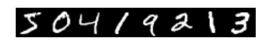
#用一行来显示前八个图像
imshow(solver.net.blobs['data'].data[:8, 0].transpose(1, 0, 2).reshape(28, 8*28), cmap='gray'); axis('off')
print 'train labels',solver.net.blobs['label'].data[:8]

train labels [ 5. 0. 4. 1. 9. 2. 1. 3.]
这里写图片描述

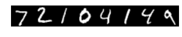
imshow(solver.test_nets[0].blobs['data'].data[:8, 0].transpose(1, 0, 2).reshape(28, 8*28), cmap='gray'); axis('off')
print 'test labels:', solver.test_nets[0].blobs['label'].data[:8]

test labels: [ 7. 2. 1. 0. 4. 1. 4. 9.]
这里写图片描述

#第三步，一步步操作去观察
solver.step(2)

imshow(solver.net.params['conv1'][0].diff[:, 0].reshape(4, 5, 5, 5).transpose(0, 2, 1, 3).reshape(4*5, 5*5), cmap='gray'); axis('off')

(-0.5, 24.5, 19.5, -0.5)
这里写图片描述

#训练网络
%time
niter = 400
test_interval = 25
# losses will also be stored in the log
train_loss = zeros(niter)
test_acc = zeros(int(np.ceil(niter / test_interval)))
output = zeros((niter, 8, 10))

# the main solver loop
for it in range(niter):
    solver.step(1)  # SGD by Caffe

    # store the train loss
    train_loss[it] = solver.net.blobs['loss'].data

    # store the output on the first test batch
    # (start the forward pass at conv1 to avoid loading new data)
    solver.test_nets[0].forward(start='conv1')
    output[it] = solver.test_nets[0].blobs['score'].data[:8]

    # run a full test every so often
    # (Caffe can also do this for us and write to a log, but we show here
    #  how to do it directly in Python, where more complicated things are easier.)
    if it % test_interval == 0:
        print 'Iteration', it, 'testing...'
        correct = 0
        for test_it in range(100):
            solver.test_nets[0].forward()
            correct += sum(solver.test_nets[0].blobs['score'].data.argmax(1)
                           == solver.test_nets[0].blobs['label'].data)
        test_acc[it // test_interval] = correct / 1e4

PU times: user 0 ns, sys: 0 ns, total: 0 ns
Wall time: 5.96 µs
Iteration 0 testing…
Iteration 25 testing…
Iteration 50 testing…
Iteration 75 testing…
Iteration 100 testing…
Iteration 125 testing…
Iteration 150 testing…
Iteration 175 testing…
Iteration 200 testing…
Iteration 225 testing…
Iteration 250 testing…
Iteration 275 testing…
Iteration 300 testing…
Iteration 325 testing…
Iteration 350 testing…
Iteration 375 testing…

_, ax1 = subplots()
ax2 = ax1.twinx()
ax1.plot(arange(niter), train_loss)
ax2.plot(test_interval * arange(len(test_acc)), test_acc, 'r')
ax1.set_xlabel('iteration')
ax1.set_ylabel('train loss')
ax2.set_ylabel('test accuracy')
ax2.set_title('Test Accuracy: {:.2f}'.format(test_acc[-1]))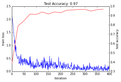

这里写图片描述

#经过最后一层raw，查看迭代次数与预估值。横坐标为迭代次数，纵坐标为预估值，其中白色表示1，黑色表示0.越白表示属于这个数的概率越大
for i in range(8):
    figure(figsize=(2, 2))
    imshow(solver.test_nets[0].blobs['data'].data[i, 0], cmap='gray')
    figure(figsize=(10, 2))
    imshow(output[:50, i].T, interpolation='nearest', cmap='gray')
    xlabel('iteration')
    ylabel('label')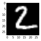

这里写图片描述

其他省略。。共计8个！

#用softmax回归来做,可以看出0，1的效果更加明显

for i in range(8):
    figure(figsize=(2, 2))
    imshow(solver.test_nets[0].blobs['data'].data[i, 0], cmap='gray')
    figure(figsize=(10, 2))
    imshow(exp(output[:50, i].T) / exp(output[:50, i].T).sum(0), interpolation='nearest', cmap='gray')
    xlabel('iteration')
    ylabel('label')

这里写图片描述


#根据已经定义好了的网络结构配置文件.prototxt和训练参数配置文件solver.prototxt文件进行训练
train_net_path = 'mnist/custom_auto_train.prototxt'
test_net_path = 'mnist/custom_auto_test.prototxt'
solver_config_path = 'mnist/custom_auto_solver.prototxt'

### define net
def custom_net(lmdb, batch_size):
    # define your own net!
    n = caffe.NetSpec()

    # keep this data layer for all networks
    n.data, n.label = L.Data(batch_size=batch_size, backend=P.Data.LMDB, source=lmdb,
                             transform_param=dict(scale=1./255), ntop=2)

    # EDIT HERE to try different networks
    # this single layer defines a simple linear classifier
    # (in particular this defines a multiway logistic regression)
    n.score =   L.InnerProduct(n.data, num_output=10, weight_filler=dict(type='xavier'))

    # EDIT HERE this is the LeNet variant we have already tried
    # n.conv1 = L.Convolution(n.data, kernel_size=5, num_output=20, weight_filler=dict(type='xavier'))
    # n.pool1 = L.Pooling(n.conv1, kernel_size=2, stride=2, pool=P.Pooling.MAX)
    # n.conv2 = L.Convolution(n.pool1, kernel_size=5, num_output=50, weight_filler=dict(type='xavier'))
    # n.pool2 = L.Pooling(n.conv2, kernel_size=2, stride=2, pool=P.Pooling.MAX)
    # n.fc1 =   L.InnerProduct(n.pool2, num_output=500, weight_filler=dict(type='xavier'))
    # EDIT HERE consider L.ELU or L.Sigmoid for the nonlinearity
    # n.relu1 = L.ReLU(n.fc1, in_place=True)
    # n.score =   L.InnerProduct(n.fc1, num_output=10, weight_filler=dict(type='xavier'))

    # keep this loss layer for all networks
    n.loss =  L.SoftmaxWithLoss(n.score, n.label)

    return n.to_proto()


with open(train_net_path, 'w') as f:
    f.write(str(custom_net('mnist/mnist_train_lmdb', 64)))    
with open(test_net_path, 'w') as f:
    f.write(str(custom_net('mnist/mnist_test_lmdb', 100)))


### define solver
from caffe.proto import caffe_pb2
s = caffe_pb2.SolverParameter()

# Set a seed for reproducible experiments:
# this controls for randomization in training.
s.random_seed = 0xCAFFE

# Specify locations of the train and (maybe) test networks.
s.train_net = train_net_path
s.test_net.append(test_net_path)
s.test_interval = 500  # Test after every 500 training iterations.
s.test_iter.append(100) # Test on 100 batches each time we test.

s.max_iter = 10000     # no. of times to update the net (training iterations)

# EDIT HERE to try different solvers
# solver types include "SGD", "Adam", and "Nesterov" among others.
s.type = "Adam"

# Set the initial learning rate for SGD.
s.base_lr = 0.01  # EDIT HERE to try different learning rates
# Set momentum to accelerate learning by
# taking weighted average of current and previous updates.
s.momentum = 0.9
# Set weight decay to regularize and prevent overfitting
s.weight_decay = 5e-4

# Set `lr_policy` to define how the learning rate changes during training.
# This is the same policy as our default LeNet.
s.lr_policy = 'inv'
s.gamma = 0.0001
s.power = 0.75
# EDIT HERE to try the fixed rate (and compare with adaptive solvers)
# `fixed` is the simplest policy that keeps the learning rate constant.
# s.lr_policy = 'fixed'

# Display the current training loss and accuracy every 1000 iterations.
s.display = 1000

# Snapshots are files used to store networks we've trained.
# We'll snapshot every 5K iterations -- twice during training.
s.snapshot = 5000
s.snapshot_prefix = 'mnist/custom_net'

# Train on the GPU
s.solver_mode = caffe_pb2.SolverParameter.GPU

# Write the solver to a temporary file and return its filename.
with open(solver_config_path, 'w') as f:
    f.write(str(s))

### load the solver and create train and test nets
solver = None  # ignore this workaround for lmdb data (can't instantiate two solvers on the same data)
solver = caffe.get_solver(solver_config_path)

### solve
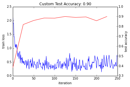
niter = 250  # EDIT HERE increase to train for longer
test_interval = niter / 10
# losses will also be stored in the log
train_loss = zeros(niter)
test_acc = zeros(int(np.ceil(niter / test_interval)))

# the main solver loop
for it in range(niter):
    solver.step(1)  # SGD by Caffe

    # store the train loss
    train_loss[it] = solver.net.blobs['loss'].data

    # run a full test every so often
    # (Caffe can also do this for us and write to a log, but we show here
    #  how to do it directly in Python, where more complicated things are easier.)
    if it % test_interval == 0:
        print 'Iteration', it, 'testing...'
        correct = 0
        for test_it in range(100):

            solver.test_nets[0].forward()
            correct += sum(solver.test_nets[0].blobs['score'].data.argmax(1)
                           == solver.test_nets[0].blobs['label'].data)
        test_acc[it // test_interval] = correct / 1e4

_, ax1 = subplots()
ax2 = ax1.twinx()
ax1.plot(arange(niter), train_loss)
ax2.plot(test_interval * arange(len(test_acc)), test_acc, 'r')
ax1.set_xlabel('iteration')
ax1.set_ylabel('train loss')
ax2.set_ylabel('test accuracy')
ax2.set_title('Custom Test Accuracy: {:.2f}'.format(test_acc[-1]))

Iteration 0 testing…
Iteration 25 testing…
Iteration 50 testing…
Iteration 75 testing…
Iteration 100 testing…
Iteration 125 testing…
Iteration 150 testing…
Iteration 175 testing…
Iteration 200 testing…
Iteration 225 testing…

这里写图片描述