sklearn_trim_PCA降维学习_菜菜视频笔记

#PCA的衡量指标是样本方差
#为什么样本方差的分母是n-1？
#简述：因为均值已经用了n个数的平均来做估计在求方差时，只有(n-1)个数和均值信息是不相关的。
#而第ｎ个数已经可以由前(n-1)个数和均值　来唯一确定，实际上没有信息量。所以在计算方差时，只除以(n-1)。

#如何“正确”的估计方差（使得样本方差接近实际总体数据的方差）
#(答案是把样本差值平方之和/n)的分母n换成n-1，通过这种方法把原来的偏小的估计“放大”一点点，我们就能获得对方差的正确估计了：

#pca与特征选择的区别，新特征矩阵不具有可读性

#2.2重要参数n_components(成分)
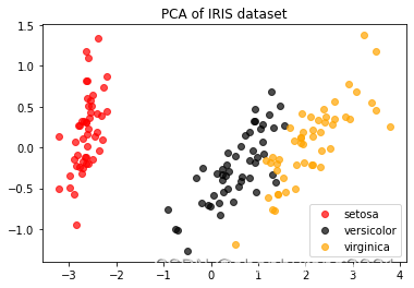
#2.2.1高维数据可视化
import matplotlib.pyplot as plt
from sklearn.datasets import load_iris
from sklearn.decomposition import PCA #降维模块

iris=load_iris()

y=iris.target
X=iris.data

X.shape

(150, 4)

import pandas as pd
pd.DataFrame(X)

	0	1	2	3
0	5.1	3.5	1.4	0.2
1	4.9	3.0	1.4	0.2
2	4.7	3.2	1.3	0.2
3	4.6	3.1	1.5	0.2
4	5.0	3.6	1.4	0.2
...	...	...	...	...
145	6.7	3.0	5.2	2.3
146	6.3	2.5	5.0	1.9
147	6.5	3.0	5.2	2.0
148	6.2	3.4	5.4	2.3
149	5.9	3.0	5.1	1.8

150 rows × 4 columns

y

array([0, 0, 0, 0, 0, 0, 0, 0, 0, 0, 0, 0, 0, 0, 0, 0, 0, 0, 0, 0, 0, 0,
       0, 0, 0, 0, 0, 0, 0, 0, 0, 0, 0, 0, 0, 0, 0, 0, 0, 0, 0, 0, 0, 0,
       0, 0, 0, 0, 0, 0, 1, 1, 1, 1, 1, 1, 1, 1, 1, 1, 1, 1, 1, 1, 1, 1,
       1, 1, 1, 1, 1, 1, 1, 1, 1, 1, 1, 1, 1, 1, 1, 1, 1, 1, 1, 1, 1, 1,
       1, 1, 1, 1, 1, 1, 1, 1, 1, 1, 1, 1, 2, 2, 2, 2, 2, 2, 2, 2, 2, 2,
       2, 2, 2, 2, 2, 2, 2, 2, 2, 2, 2, 2, 2, 2, 2, 2, 2, 2, 2, 2, 2, 2,
       2, 2, 2, 2, 2, 2, 2, 2, 2, 2, 2, 2, 2, 2, 2, 2, 2, 2])

pca=PCA(n_components=2)
X_dr=pca.fit_transform(X)

X_dr

array([[-2.68412563,  0.31939725],
       [-2.71414169, -0.17700123],
       [-2.88899057, -0.14494943],
       [-2.74534286, -0.31829898],
       [-2.72871654,  0.32675451],
       [-2.28085963,  0.74133045],
       [-2.82053775, -0.08946138],
       [-2.62614497,  0.16338496],
       [-2.88638273, -0.57831175],
       [-2.6727558 , -0.11377425],
       [-2.50694709,  0.6450689 ],
       [-2.61275523,  0.01472994],
       [-2.78610927, -0.235112  ],
       [-3.22380374, -0.51139459],
       [-2.64475039,  1.17876464],
       [-2.38603903,  1.33806233],
       [-2.62352788,  0.81067951],
       [-2.64829671,  0.31184914],
       [-2.19982032,  0.87283904],
       [-2.5879864 ,  0.51356031],
       [-2.31025622,  0.39134594],
       [-2.54370523,  0.43299606],
       [-3.21593942,  0.13346807],
       [-2.30273318,  0.09870885],
       [-2.35575405, -0.03728186],
       [-2.50666891, -0.14601688],
       [-2.46882007,  0.13095149],
       [-2.56231991,  0.36771886],
       [-2.63953472,  0.31203998],
       [-2.63198939, -0.19696122],
       [-2.58739848, -0.20431849],
       [-2.4099325 ,  0.41092426],
       [-2.64886233,  0.81336382],
       [-2.59873675,  1.09314576],
       [-2.63692688, -0.12132235],
       [-2.86624165,  0.06936447],
       [-2.62523805,  0.59937002],
       [-2.80068412,  0.26864374],
       [-2.98050204, -0.48795834],
       [-2.59000631,  0.22904384],
       [-2.77010243,  0.26352753],
       [-2.84936871, -0.94096057],
       [-2.99740655, -0.34192606],
       [-2.40561449,  0.18887143],
       [-2.20948924,  0.43666314],
       [-2.71445143, -0.2502082 ],
       [-2.53814826,  0.50377114],
       [-2.83946217, -0.22794557],
       [-2.54308575,  0.57941002],
       [-2.70335978,  0.10770608],
       [ 1.28482569,  0.68516047],
       [ 0.93248853,  0.31833364],
       [ 1.46430232,  0.50426282],
       [ 0.18331772, -0.82795901],
       [ 1.08810326,  0.07459068],
       [ 0.64166908, -0.41824687],
       [ 1.09506066,  0.28346827],
       [-0.74912267, -1.00489096],
       [ 1.04413183,  0.2283619 ],
       [-0.0087454 , -0.72308191],
       [-0.50784088, -1.26597119],
       [ 0.51169856, -0.10398124],
       [ 0.26497651, -0.55003646],
       [ 0.98493451, -0.12481785],
       [-0.17392537, -0.25485421],
       [ 0.92786078,  0.46717949],
       [ 0.66028376, -0.35296967],
       [ 0.23610499, -0.33361077],
       [ 0.94473373, -0.54314555],
       [ 0.04522698, -0.58383438],
       [ 1.11628318, -0.08461685],
       [ 0.35788842, -0.06892503],
       [ 1.29818388, -0.32778731],
       [ 0.92172892, -0.18273779],
       [ 0.71485333,  0.14905594],
       [ 0.90017437,  0.32850447],
       [ 1.33202444,  0.24444088],
       [ 1.55780216,  0.26749545],
       [ 0.81329065, -0.1633503 ],
       [-0.30558378, -0.36826219],
       [-0.06812649, -0.70517213],
       [-0.18962247, -0.68028676],
       [ 0.13642871, -0.31403244],
       [ 1.38002644, -0.42095429],
       [ 0.58800644, -0.48428742],
       [ 0.80685831,  0.19418231],
       [ 1.22069088,  0.40761959],
       [ 0.81509524, -0.37203706],
       [ 0.24595768, -0.2685244 ],
       [ 0.16641322, -0.68192672],
       [ 0.46480029, -0.67071154],
       [ 0.8908152 , -0.03446444],
       [ 0.23054802, -0.40438585],
       [-0.70453176, -1.01224823],
       [ 0.35698149, -0.50491009],
       [ 0.33193448, -0.21265468],
       [ 0.37621565, -0.29321893],
       [ 0.64257601,  0.01773819],
       [-0.90646986, -0.75609337],
       [ 0.29900084, -0.34889781],
       [ 2.53119273, -0.00984911],
       [ 1.41523588, -0.57491635],
       [ 2.61667602,  0.34390315],
       [ 1.97153105, -0.1797279 ],
       [ 2.35000592, -0.04026095],
       [ 3.39703874,  0.55083667],
       [ 0.52123224, -1.19275873],
       [ 2.93258707,  0.3555    ],
       [ 2.32122882, -0.2438315 ],
       [ 2.91675097,  0.78279195],
       [ 1.66177415,  0.24222841],
       [ 1.80340195, -0.21563762],
       [ 2.1655918 ,  0.21627559],
       [ 1.34616358, -0.77681835],
       [ 1.58592822, -0.53964071],
       [ 1.90445637,  0.11925069],
       [ 1.94968906,  0.04194326],
       [ 3.48705536,  1.17573933],
       [ 3.79564542,  0.25732297],
       [ 1.30079171, -0.76114964],
       [ 2.42781791,  0.37819601],
       [ 1.19900111, -0.60609153],
       [ 3.49992004,  0.4606741 ],
       [ 1.38876613, -0.20439933],
       [ 2.2754305 ,  0.33499061],
       [ 2.61409047,  0.56090136],
       [ 1.25850816, -0.17970479],
       [ 1.29113206, -0.11666865],
       [ 2.12360872, -0.20972948],
       [ 2.38800302,  0.4646398 ],
       [ 2.84167278,  0.37526917],
       [ 3.23067366,  1.37416509],
       [ 2.15943764, -0.21727758],
       [ 1.44416124, -0.14341341],
       [ 1.78129481, -0.49990168],
       [ 3.07649993,  0.68808568],
       [ 2.14424331,  0.1400642 ],
       [ 1.90509815,  0.04930053],
       [ 1.16932634, -0.16499026],
       [ 2.10761114,  0.37228787],
       [ 2.31415471,  0.18365128],
       [ 1.9222678 ,  0.40920347],
       [ 1.41523588, -0.57491635],
       [ 2.56301338,  0.2778626 ],
       [ 2.41874618,  0.3047982 ],
       [ 1.94410979,  0.1875323 ],
       [ 1.52716661, -0.37531698],
       [ 1.76434572,  0.07885885],
       [ 1.90094161,  0.11662796],
       [ 1.39018886, -0.28266094]])

X_dr.shape

(150, 2)

y==0

array([ True,  True,  True,  True,  True,  True,  True,  True,  True,
        True,  True,  True,  True,  True,  True,  True,  True,  True,
        True,  True,  True,  True,  True,  True,  True,  True,  True,
        True,  True,  True,  True,  True,  True,  True,  True,  True,
        True,  True,  True,  True,  True,  True,  True,  True,  True,
        True,  True,  True,  True,  True, False, False, False, False,
       False, False, False, False, False, False, False, False, False,
       False, False, False, False, False, False, False, False, False,
       False, False, False, False, False, False, False, False, False,
       False, False, False, False, False, False, False, False, False,
       False, False, False, False, False, False, False, False, False,
       False, False, False, False, False, False, False, False, False,
       False, False, False, False, False, False, False, False, False,
       False, False, False, False, False, False, False, False, False,
       False, False, False, False, False, False, False, False, False,
       False, False, False, False, False, False, False, False, False,
       False, False, False, False, False, False])

colors=['red','black','orange']

plt.figure()
for i in[0,1,2]:
    plt.scatter(X_dr[y==i,0]
                ,X_dr[y==i,1]
                ,alpha=.7
                ,c=colors[i]
                ,label=iris.target_names[i]
               )
plt.legend()#画图例
plt.title('PCA of IRIS dataset')
plt.show()

pca.explained_variance_#(信息量，可解释性方差） 

array([4.22824171, 0.24267075])

pca.explained_variance_ratio_#特征在原数据的信息占比

array([0.92461872, 0.05306648])

pca.explained_variance_ratio_.sum()#特征在原数据的信息占比总和

0.9776852063187949

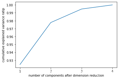
pca_line=PCA().fit(X)
pca_line.explained_variance_ratio_#查看原数据特征信息占比

array([0.92461872, 0.05306648, 0.01710261, 0.00521218])

import numpy as np
np.cumsum(pca_line.explained_variance_ratio_)

array([0.92461872, 0.97768521, 0.99478782, 1.        ])

pac_line=PCA().fit(X)
plt.plot([1,2,3,4],np.cumsum(pca_line.explained_variance_ratio_))
plt.xticks([1,2,3,4])#使得坐标轴显示为整数
plt.xlabel("number of components after dimension reduction")
plt.ylabel("cumulative explained variance ratip")
plt.show()

pca_mle=PCA(n_components='mle')
pca_mle=pca_mle.fit(X)

X_mle=pca_mle.transform(X)

X_mle.shape

(150, 3)

pca_mle.explained_variance_ratio_.sum()

0.9947878161267246

#2.2.3 按信息占比选超参数
pca_f=PCA(n_components=0.97,svd_solver='full')
pca_f=pca_f.fit(X)
X_f=pca_f.transform(X)
pca_f.explained_variance_ratio_

array([0.92461872, 0.05306648])

pca_f.explained_variance_ratio_.sum()

0.9776852063187949

#2.3PCA中的SVD
#2.3.1PCA中的SVD哪里来？
#奇异值分解跳过计算协方差矩阵直接求出新空间（空间转换矩阵）和降维后的特征矩阵
#在矩阵分解时不使用PCA本身的特征值分解，而使用奇异值分解来减少计算量，奇异值分解产生的V（k,n）保存于属性componenets_

PCA(2).fit(X).components_

array([[ 0.36138659, -0.08452251,  0.85667061,  0.3582892 ],
       [ 0.65658877,  0.73016143, -0.17337266, -0.07548102]])

PCA(2).fit(X).components_.shape#降维后的新特征空间

(2, 4)

#2.3.2svd_solver与random_state
#full：根据原始数据和n_components计算寻找特征向量，完整的生成SVD的三个结构
#auto:如果数据大于500*500且特征数小于数据最小维度80%，就启用randomized截断会在矩阵被分解后有选择的发生
#arpack:适用于高维的稀疏矩阵，加快分解速度
#randomized:适用于巨大矩阵，计算量大；分解器生成随机向量，检测是否符合需求，如果符合，保留随机向量，基于此构建后续向量空间

#random_state在参数svd_solver为'arpack'or'randomized'

#如果特征空间是图像，空间矩阵能够可视化

from sklearn.datasets import fetch_lfw_people
from sklearn.decomposition import PCA
import matplotlib.pyplot as plt
import numpy as np

faces=fetch_lfw_people(min_faces_per_person=60)#实例化

faces.data.shape#降维支持小于二维特征，（images形式）

(1348, 2914)

faces.images.shape#1348是图像个数，62，47分别是特征矩阵的行列

(1348, 62, 47)

X=faces.data

fig,axes=plt.subplots(4,5
                      ,figsize=(8,4)
                      ,subplot_kw={"xticks":[],"yticks":[]}
                     )
axes[0][0].imshow(faces.images[0,:,:])#轴图像（子画布）

<matplotlib.image.AxesImage at 0x1d6b4480c70>

axes.shape

(4, 5)

axes[0][0].imshow(faces.images[0,:,:])

<matplotlib.image.AxesImage at 0x1d6b44803a0>

axes.flat

<numpy.flatiter at 0x1d6add0a890>

([*axes.flat])

[<AxesSubplot:>,
 <AxesSubplot:>,
 <AxesSubplot:>,
 <AxesSubplot:>,
 <AxesSubplot:>,
 <AxesSubplot:>,
 <AxesSubplot:>,
 <AxesSubplot:>,
 <AxesSubplot:>,
 <AxesSubplot:>,
 <AxesSubplot:>,
 <AxesSubplot:>,
 <AxesSubplot:>,
 <AxesSubplot:>,
 <AxesSubplot:>,
 <AxesSubplot:>,
 <AxesSubplot:>,
 <AxesSubplot:>,
 <AxesSubplot:>,
 <AxesSubplot:>]

len([*axes.flat])#[*]打开惰性对象，.flat降维

20

#填充函数

[*enumerate(axes.flat)]#enumerate形成元组

[(0, <AxesSubplot:>),
 (1, <AxesSubplot:>),
 (2, <AxesSubplot:>),
 (3, <AxesSubplot:>),
 (4, <AxesSubplot:>),
 (5, <AxesSubplot:>),
 (6, <AxesSubplot:>),
 (7, <AxesSubplot:>),
 (8, <AxesSubplot:>),
 (9, <AxesSubplot:>),
 (10, <AxesSubplot:>),
 (11, <AxesSubplot:>),
 (12, <AxesSubplot:>),
 (13, <AxesSubplot:>),
 (14, <AxesSubplot:>),
 (15, <AxesSubplot:>),
 (16, <AxesSubplot:>),
 (17, <AxesSubplot:>),
 (18, <AxesSubplot:>),
 (19, <AxesSubplot:>)]

fig,axes=plt.subplots(3,8
                      ,figsize=(8,4)
                      ,subplot_kw={"xticks":[],"yticks":[]}
                     )
for i,ax in enumerate(axes.flat):
    ax.imshow(faces.images[i,:,:]
             ,cmap="gray")

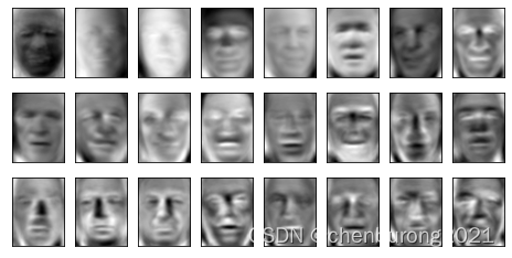
#4.降维，提取特征空间

pca=PCA(150).fit(X)

V=pca.components_#V(k,n)保存在属性components_中:新特征矩阵,转化矩阵，可以将原特征矩阵转化新矩阵
V.shape

(150, 2914)

fig,axes=plt.subplots(3,8
                      ,figsize=(8,4)
                      ,subplot_kw={"xticks":[],"yticks":[]}
                     )
for i,ax in enumerate(axes.flat):
    ax.imshow(V[i,:].reshape(62,47)#一维特征升二维特征，形式改变可视化
             ,cmap="gray")
#显示了新特征空间的特点，新特征为重要数据[五官，明暗分布]

pca=PCA(150)
X_dr=pca.fit_transform(X)
X_dr.shape
#获得新特征

(1348, 150)

X_inverse=pca.inverse_transform(X_dr )
X_inverse.shape
#将新特征导回原空间，升维，图像于原图像高度相似，但是信息仍损失，图片变模糊，所以降维是不可逆的

(1348, 2914)

fig,ax=plt.subplots(2,10,figsize=(10,2.5)
                      ,subplot_kw={"xticks":[],"yticks":[]}
                     )
for i in range(10):
    ax[0,i].imshow(faces.images[i,:,:],cmap="binary_r")
    ax[1,i].imshow(X_inverse[i].reshape(62,47),cmap="binary_r")

ax[0,1]

<AxesSubplot:>

faces.images.shape

(1348, 62, 47)

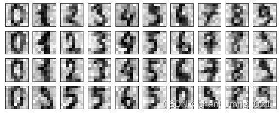
#2.4.2PCA做噪音过滤

from sklearn.datasets import load_digits
from sklearn.decomposition import PCA
import matplotlib.pyplot as plt
import numpy as np

digits=load_digits()

digits.data.shape

(1797, 64)

set(digits.target.tolist())#去重

{0, 1, 2, 3, 4, 5, 6, 7, 8, 9}

digits.images.shape

(1797, 8, 8)

def plot_digits(data):#设置封装接口
    fig,axes=plt.subplots(4,10,figsize=(10,4)
                      ,subplot_kw={"xticks":[],"yticks":[]}
                     )
    for i,ax in enumerate(axes.flat):
        ax.imshow(data[i].reshape(8,8),cmap="binary")

plot_digits(digits.data)

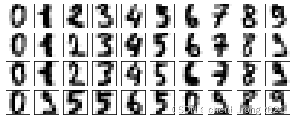
import numpy as np
rng=np.random.RandomState(42) #规定随机模式
noisy=rng.normal(digits.data,2)#从中随机抽取满足正态分布的另一个数据集，剥离创造，和设置抽取正态分布的标准差

noisy.shape#(同原数据结构)

(1797, 64)

plot_digits(noisy)

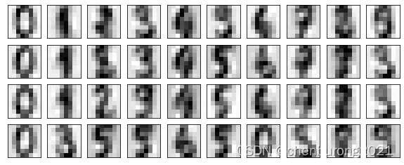
pca=PCA(0.5,svd_solver="full").fit(noisy)#获得大量有效特征
X_dr=pca.transform(noisy)

X_dr.shape

(1797, 6)

without_noise=pca.inverse_transform(X_dr)

without_noise.shape

(1797, 64)

plot_digits(without_noise)

#重要参数
#n_components：成分，svd_solver：svd处理方法，randomized控制拥有随机模型的处理方法

#三个重要属性
#components：V(k,n)保存在属性components_中:转化矩阵；
#explained_variance:解释性特征
#explained_variance_ratio：解释性特征信息占比

#接口inverse_transform，降维恢复(信息仍损失)#将降维后数据返回原特征空间

#没啥用，计算协方差矩阵并计算get_covariance