


目录
1. 前言
在前一篇中MobileNets(V1)简介及两个初步的代码实验介绍基于Tensorflow.keras的预训练模型的实验,本篇更进一步,直接搭建一个MobileNetV1网络模型并在Cifar10数据集上从零开始训练。MobileNetV1网络模型的代码参考自另一篇CSDN博客(Ref2)。
2. 模型搭建
import tensorflow as tf
from tensorflow import keras
from tensorflow.keras import layers
from tensorflow.keras import utils
import numpy as np
import matplotlib.pyplot as plt
from PIL import Image
print(tf.__version__)

def conv_block(inputs,filters,kernel_size=(3, 3),strides=(1, 1)):
    x = tf.keras.layers.Conv2D(filters, kernel_size=kernel_size, strides=strides, padding='same', use_bias=False)(
        inputs)
    tf.keras.layers.BatchNormalization()(x)
    return tf.keras.layers.ReLU(6.0)(x)

def depthwise_conv_block(inputs,pointwise_conv_filters,strides=(1, 1)):
    x = tf.keras.layers.DepthwiseConv2D((3, 3), padding='same', strides=strides, use_bias=False)(inputs)
    x = tf.keras.layers.BatchNormalization()(x)
    x = tf.keras.layers.ReLU(6.0)(x)

    x = tf.keras.layers.Conv2D(pointwise_conv_filters, kernel_size=(1, 1), padding='same', use_bias=False)(x)
    x = tf.keras.layers.BatchNormalization()(x)

    return tf.keras.layers.ReLU(6.0)(x)

def mobilenet_v1(inputs,classes):
    x = conv_block(inputs, 32, strides=(2, 2))
    x = depthwise_conv_block(x, 64)
    x = depthwise_conv_block(x, 128, strides=(2, 2))
    x = depthwise_conv_block(x, 128)
    x = depthwise_conv_block(x, 256, strides=(2, 2))
    x = depthwise_conv_block(x, 256)
    x = depthwise_conv_block(x, 512, strides=(2, 2))
    x = depthwise_conv_block(x, 512)
    x = depthwise_conv_block(x, 512)
    x = depthwise_conv_block(x, 512)
    x = depthwise_conv_block(x, 512)
    x = depthwise_conv_block(x, 512)
    x = depthwise_conv_block(x, 1024, strides=(2, 2))
    x = depthwise_conv_block(x, 1024)
    x = tf.keras.layers.GlobalAveragePooling2D()(x)
    x = tf.keras.layers.Dense(classes, activation='softmax')(x)
    return x

INPUT_WIDTH = 32
INPUT_HEIGHT = 32
N_CHANNELS = 3
N_CLASSES = 10
inputs = tf.keras.Input(shape=(INPUT_WIDTH, INPUT_HEIGHT, N_CHANNELS))
model = tf.keras.Model(inputs=inputs, outputs=mobilenet_v1(inputs, N_CLASSES))
model.summary()
相比常规的卷积神经网络,就是多出来tf.keras.layers.DepthwiseConv2D的调用。当然,更进一步的话,也可以纯粹地基于python/numpy来实现自己的DepthwiseConv2D。
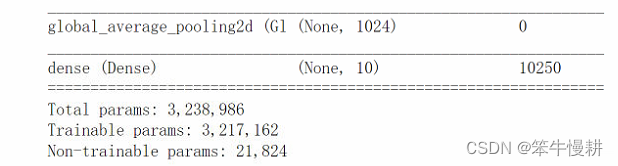
总参数个数与上一篇中基于预训练模型的结构的参数个数略有出入(少了64个参数,why?),待确认。
3. 数据准备
基于tensorflow.keras内置数据集cifar10进行实验。
(x_train, y_train), (x_test, y_test) = tf.keras.datasets.cifar10.load_data()
x_train = x_train / 255.0
y_train = tf.keras.utils.to_categorical(y_train, N_CLASSES)
x_test  = x_test / 255.0
y_test  = tf.keras.utils.to_categorical(y_test, N_CLASSES)
4. 模型训练
from tensorflow.keras import optimizers
model.compile(loss="categorical_crossentropy",
    #optimizer=optimizers.RMSprop(learning_rate=2e-5),
    optimizer='RMSprop',
    #metrics=['categorical_accuracy', 'Recall', 'AUC'])
    metrics=['accuracy', 'Recall', 'AUC'])

callbacks = [
    keras.callbacks.ModelCheckpoint(
      filepath="mobilenet_v1_cifar10.h5",
      save_best_only=True,
      monitor="val_loss")
]
history = model.fit(
    x_train, y_train,
    batch_size=32,
    epochs=20,
    validation_data=(x_test, y_test),
    callbacks=callbacks)
5. 结果分析
import matplotlib.pyplot as plt
accuracy = history.history["accuracy"]
val_accuracy = history.history["val_accuracy"]
loss = history.history["loss"]
val_loss = history.history["val_loss"]
epochs = range(1, len(accuracy) + 1)
fig,ax = plt.subplots(1,2,figsize=(12,6)) # figsize=(width, height)
ax[0].plot(epochs, accuracy, "bo", label="Training accuracy")
ax[0].plot(epochs, val_accuracy, "b", label="Validation accuracy")
ax[0].set_title("Training and validation accuracy")
ax[0].legend()
ax[1].plot(epochs, loss, "bo", label="Training loss")
ax[1].plot(epochs, val_loss, "b", label="Validation loss")
ax[1].set_title("Training and validation loss")
ax[1].legend()
20个epoch的训练结果如下所示。
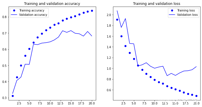
只看训练集的结果的话,再增加epoches次数应该还能进一步提高。但是看验证集上的结果的话,大概从第13轮开始就到顶进入平层了,也就是说存在比较严重的overfitting。
用基于内置MobileNetV1结构进行基于Cifar10的相同参数的训练后得到的结果如下:
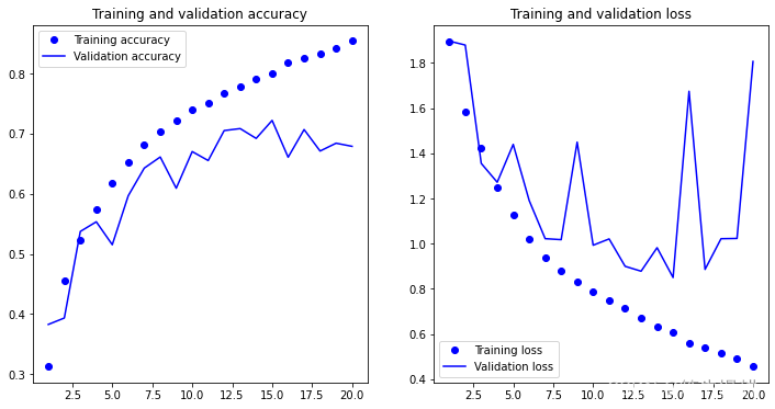
可以看到accuracy时基本一致的,但是validation loss曲线有一些差异,原因待查。
Ref1:MobileNets(V1)简介及两个初步的代码实验
Ref2: 【TensorFlow2.0实战】基于TnesorFlow实现MobileNet V1


 1261
1261

 被折叠的 条评论
为什么被折叠?
被折叠的 条评论
为什么被折叠?
 到【灌水乐园】发言


