A simple svm and some notebook

 有关svm的例子和笔记

'''from sklearn import svm
X = [[2,0],[1,1],[2,3],[2,2]]
y = [0,0,0,1]
clf = svm.SVC(kernel = 'linear')
clf.fit(X,y)
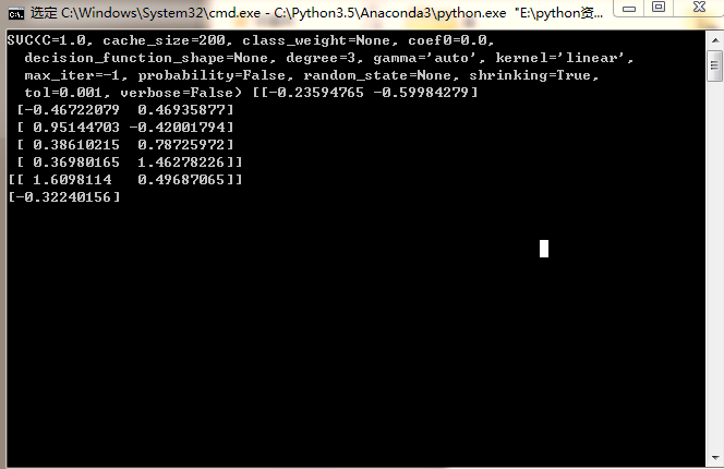
print (clf)
print (clf.support_vectors_)#训练样本中所有的支持向量
print (clf.support_)#支持向量在训练样本中的索引
print (clf.n_support_)#各类中支持向量的个数
print (clf.predict([[2,0]]))
'''
#---------------------numpy------------
import numpy as np
from sklearn import svm
import pylab as pl
#rand(2,4,2)产生2个4行2列的矩阵，数值在[0.1)之间
#randn(2,4,2) - [2,1]产生2个4行2列的标准正态分布矩阵,均值为2，方差为1，-为位于正态分布的左方np.random.seed(0)
np.random.seed(0)
X = np.r_[np.random.randn(20,2)-[2,1],np.random.randn(20,2)+[2,1]]
y = [0]*20+[1]*20
clf = svm.SVC(kernel = 'linear')
clf.fit(X,y)
print (clf,clf.support_vectors_)    
print (clf.coef_) #coef_是回归系数
print (clf.intercept_)#intercept_是截距
#y = -(w[0]/w[1])x + (w[3]/w[1])
w = clf.coef_[0]
k = -(w[0]/w[1])
xx = np.linspace(-5,5)
yy = k*xx - (clf.intercept_[0])/w[1]
b_down = clf.support_vectors_[0]
yy_down = k*xx +b_down[1]-k*b_down[0]
b_up = clf.support_vectors_[-1]
yy_up = k*xx +b_up[1]-k*b_up[0]
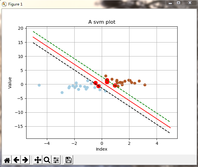
pl.plot(xx,yy,'r-')
pl.plot(xx,yy_up,'g--')
pl.plot(xx,yy_down,'k--')
pl.scatter(X[:,0],X[:,1],c=y,cmap=pl.cm.Paired)#cm即colormap，c=y表示颜色随y变化，也可以使用c=x，使得颜色随x映射
pl.scatter(clf.support_vectors_[:,0],clf.support_vectors_[:,1],s=85,color='red')#取出支持向量X和Y的值画出散点图

pl.axis('tight')#坐标轴适应数据量
pl.grid(True)#显示格子
pl.xlabel('Index')
pl.ylabel('Value')
pl.title('A svm plot')
pl.show()

# x = np.r_['0,3,1',[[1,2,3],[7,8,9]],[[4,5,6],[10,11,12]] ] #'3',是提升后的维度，
# print (x)
# y = np.random.randn(20,2)
# print (y)
# print ('\t1.\n2.\n3.')
# import numpy as np
# a = np.zeros((2,2))
# a = np.ones((2,2))
# a = np.empty((2,2))
# a = np.arange(12).reshape((3,4))
# a = np.linspace(1,10,5)
# a = np.sin([1,2])
# a = np.dot([[1,2,3],[2,1,3]],[[1,2],[3,4],[5,6]])#点积
# print(a)
# print (np.argmin(a))#axis维度
# print (np.argmax(a))#axis维度
# a = [1,2,3]
# b =[4,5,6]
# c = np.vstack((a,b))#上下合并
# c = np.r_['0,2,0',a,b]#
# # c = np.hstack((a,b))#左右合并
# print (c)
# _*_ coding : utf-8 _*_
# import pylab as pl
# from pylab import *
# mpl.rcParams['font.sans-serif'] = ['SimHei'] 
# x = range(10)
# y = [i*i for i in x]
# pl.plot(x,y,'or--',label ='y=x^2曲线图')
# pl.legend()
# pl.xlabel('横坐标')
# pl.ylabel('纵坐标')
# pl.title('y=x^2')

# pl.show()

结果如下：

转载于:https://my.oschina.net/u/3786144/blog/1799184