最小二乘法求解一元线性回归

最小二乘法求解一元线性回归

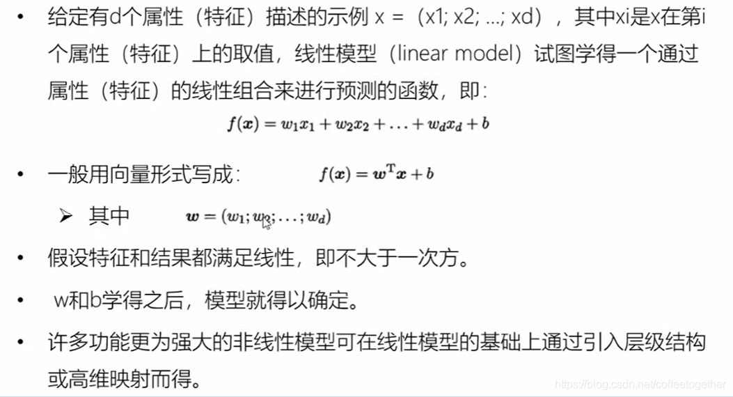
介绍线性回归模型以及简单一元线性回归模型的解法。

通过代码实现最小二乘法求解一元线性回归实例，并对结果进行预测。

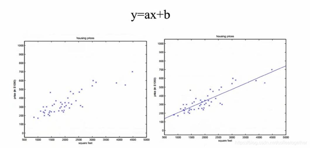
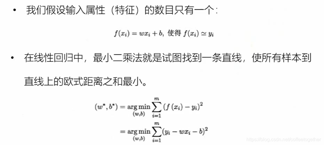
一、线性回归

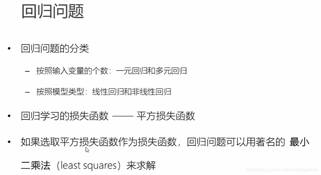
二、回归问题的解决

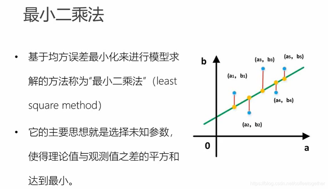
三、最小二乘法介绍

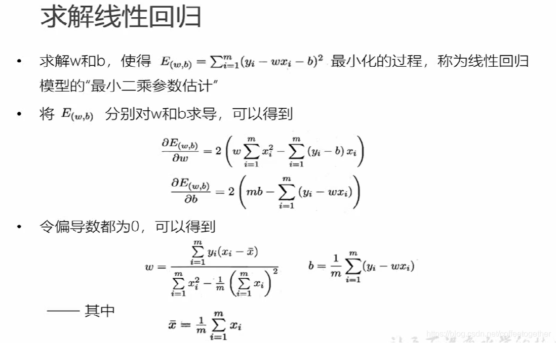
四、最小二乘法求解线性回归

五、实例验证

案例背景：数据中参数x为学习时间，y为得分。通过最小二乘法求解参数w，b，均方差。并预测x=80时的得分。

数据链接：
链接: https://pan.baidu.com/s/1KVw_9O5o9vqQnpgRNfLGVQ
提取码：8u8e

1.导入数据

# 导入必要库
import numpy as np
import matplotlib.pyplot as plt

points = np.genfromtxt('E:/PythonData/machine_learning/data.csv',delimiter=',')

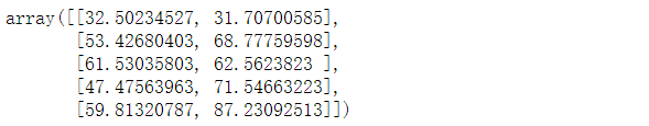
# 查看前5行数据
points[:5]

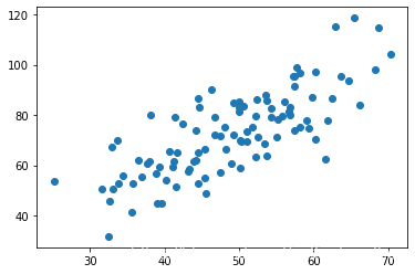
2.绘制散点图

# 分别提取points中的x和y数据
x = points[:,0]
y = points[:,1]

# 绘制散点图
plt.scatter(x,y)
plt.show()

3.定义损失函数

# 损失函数是系数w，b的函数，另外还要传入数据x，y
def computer_cost(w,b,points):
    total_cost = 0
    M = len(points)
  
    # 逐点计算平方损失误差，然后求平均数
    for i in range(M):
        x = points[i,0]
        y = points[i,1]
        total_cost +=(y - w *x - b)**2
    # 取平均
    return total_cost/M

4.定义算法拟合函数

# 先定义求均值函数
def average(data):
    sum = 0
    num = len(data)
    for i in range(num):
        sum+=data[i]
    return sum/num
    
# 定义核心拟合函数
def fit(points):
    M = len(points)
    x_bar = average(points[:,0])
    
    sum_yx = 0
    sum_x2 = 0
    sum_delta = 0
    
    for i in range(M):
        x = points[i,0]
        y = points[i,1]
        sum_yx += y*(x-x_bar)
        sum_x2 += x**2
        
    # 根据公式计算w
    w = sum_yx/(sum_x2 - M*(x_bar**2))
    
    # 再次创建for循环计算b
    for i in range(M):
        x = points[i,0]
        y = points[i,1]
        sum_delta += y-w*x
    b = sum_delta/M
    return w,b 

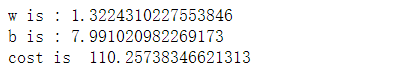
5.测试（得到参数w，b，均方误差）

# 将测试集传入拟合函数中
w,b = fit(points)
print('w is :',w)
print('b is :',b)

cost = computer_cost(w,b,points)
print('cost is ',cost)

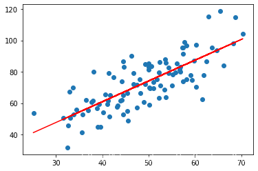
6.绘制拟合曲线

plt.scatter(x,y)

# 针对每一个x，绘制出预测的值
pred_y = w*x+b

# 画出拟合曲线，颜色设置为红色
plt.plot(x,pred_y,c='r')

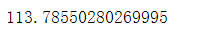
7.预测分数

# 给出参数x，得出预测结果
pred_y1 = w*80+b
print(pred_y1)