uva1356 - Bridge 自适应simpson公式

最新推荐文章于 2018-08-03 18:06:51 发布

小小小小葱

最新推荐文章于 2018-08-03 18:06:51 发布

阅读量660

点赞数

分类专栏：数学

本文链接：https://blog.csdn.net/corncsd/article/details/38469621

版权

数学专栏收录该内容

46 篇文章 0 订阅

订阅专栏

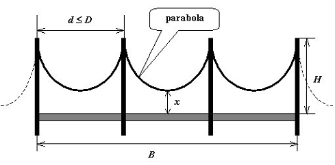
A suspension bridge suspends the roadway from huge main cables, which extend from one end of the bridge to the other. These cables rest on top of high towers and are secured at each end by anchorages. The towers enable the main cables to be draped over long distances.

Suppose that the maximum distance between two neighboring towers is D, and that the distance from the top of a tower to the roadway is H. Also suppose that the shape of a cable between any two neighboring towers is the same symmetric parabola (as shown in the figure). Now given B, the length of the bridge and L, the total length of the cables, you are asked to calculate the distance between the roadway and the lowest point of the cable, with minimum number of towers built (Assume that there are always two towers built at the two ends of a bridge).

$\epsfbox{p3485.eps}$

Input

Standard input will contain multiple test cases. The first line of the input is a single integer T (1 $\le$ T $\le$ 10) which is the number of test cases. T test cases follow, each preceded by a single blank line.

For each test case, 4 positive integers are given on a single line.

- the maximum distance between two neighboring towers;

- the distance from the top of a tower to the roadway;

- the length of the bridge; and

- the total length of the cables.

It is guaranteed that B $\le$ L. The cable will always be above the roadway.

Output

Results should be directed to standard output. Start each case with "Case #:" on a single line, where # is the case number starting from 1. Two consecutive cases should be separated by a single blank line. No blank line should be produced after the last test case.

For each test case, print the distance between the roadway and the lowest point of the cable, as is described in the problem. The value must be accurate up to two decimal places.

Sample Input

2

20 101 400 4042

1 2 3 4

Sample Output

Case 1:
1.00

Case 2:
1.60

桥上摆放等距的塔，塔高H，相邻的塔距离不超过D，塔之间绳子是抛物线。桥长B，绳子总长L，求建最少的塔时绳子下端离地的高度。

塔数目最小时，间隔数为ceil(B/D)，每个间隔的宽度D1=B/n，每段绳子长L1=L/n。设每段绳子宽度为w，高h，抛物线方程f(x)=ax^2=4h/(w^2)，二分枚举h，知道算出的抛物线长度为L1，最后答案就是H-h。

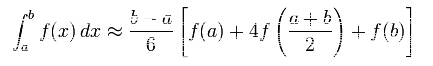
问题就在于抛物线长度怎么算。弧长积分公式∫a到b√（1+(f'(x))^2），可以积出来，但是不会积的话就可以用simpson公式。

递归算左右两部分的simpson值，如果和整体的simpson值误差小到一定精度就返回。

有一点不明白的是白书上的那个误差小于15eps就返回L+R+误差/15，为什么这样就能保证误差小于eps。。

#include<iostream>
#include<algorithm>
#include<queue>
#include<cstdio>
#include<cstdlib>
#include<cmath>
#include<cstring>
#include<stack>
#define INF 0x3f3f3f3f
#define MAXN 10010
#define MAXM 110
#define MOD 1000000007
#define MAXNODE 4*MAXN
//#define eps 1e-9
using namespace std;
typedef long long LL;
int T,D,B,H,L;
double a;
//simpson公式用到的函数
double F(double x) {
  return sqrt(1+4*a*a*x*x);
}
//三点simpson法。这里要求F是一个全局函数
double simpson(double a, double b) {
  double c=a+(b-a)/2;
  return (F(a)+4*F(c)+F(b))*(b-a)/6;
}
//自适应Simpson公式（递归过程）。已知整个区间[a,b]上的三点simpson值A
double asr(double a, double b, double eps, double A) {
  double c= a+(b-a)/2;
  double L=simpson(a,c),R=simpson(c,b);
  if(fabs(L+R-A)<=15*eps) return L+R+(L+R-A)/15;
  return asr(a,c,eps/2,L) + asr(c,b,eps/2,R);
}
//自适应Simpson公式（主过程）
double asr(double a,double b,double eps) {
  return asr(a,b,eps,simpson(a,b));
}

// 用自适应Simpson公式计算宽度为w，高度为h的抛物线长
double parabola_arc_length(double w, double h) {
  a=4.0*h/(w*w); // 修改全局变量a，从而改变全局函数F的行为
  return asr(0,w/2,1e-9)*2;
}
int main(){
    freopen("in.txt","r",stdin);
    int cas=0;
    scanf("%d",&T);
    while(T--){
        scanf("%d%d%d%d",&D,&H,&B,&L);
        int n=(B+D-1)/D;
        double D1=(double)B/n,L1=(double)L/n,l=0,r=H;
        while(r-l>1e-9){
            double mid=l+(r-l)/2;
            if(parabola_arc_length(D1,mid)<L1) l=mid;
            else r=mid;
        }
        printf("Case %d:\n%.2lf\n",++cas,H-l);
        if(T) puts("");
    }
    return 0;
}