excel vlookup_Excel VLOOKUP到左侧

excel vlookup

To use VLOOKUP, the value you're looking for has to be in the first column of the lookup range. But what if your lookup table has Scores in column 3, and you need a description from column 2? Here's how you can do an Excel VLOOKUP to the left.

要使用VLOOKUP，要查找的值必须在查找范围的第一列中。 但是，如果您的查询表在第3列中有“分数”，并且您需要在第2列中有描述，该怎么办？ 这是在左侧执行Excel VLOOKUP的方法。

查找表 (Lookup Table)

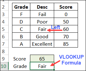
In the lookup table below, there are 3 columns, with letter grades, descriptions, and numeric scores.

在下面的查找表中，共有3列，包括字母等级，描述和数字分数。

A score is entered in cell C9, and we want our VLOOKUP formula to get the description from column C, using an approximate match for a Score.

在单元格C9中输入一个分数，我们希望VLOOKUP公式使用分数的近似匹配项从C列获取描述。

从选择中获取帮助 (Get Help from CHOOSE)

To get the VLOOKUP to work, we'll combine it with the CHOOSE function.

为了使VLOOKUP正常工作，我们将其与CHOOSE函数结合使用。

Usually, CHOOSE makes a simple selection from a list of options, such as finding the Fiscal Month, based on calendar month number.

通常，CHOOSE从选项列表中进行简单选择，例如根据日历月号查找“财政月” 。

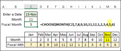
For example, if the fiscal year starts in July (month 7), the fiscal months for January to December are in this order: 7,8,9,10,11,12,1,2,3,4,5,6

例如，如果会计年度从7月(第7个月)开始，则1月至12月的会计月份的顺序为： 7,8,9,10,11,12,1,2,3,4,5,6

If we put that list of values in a CHOOSE formula, we can find the fiscal month number for the date in cell C6.

如果将值列表放入CHOOSE公式中，则可以在单元格C6中找到该日期的会计月份数字。

=CHOOSE(MONTH(C6), 7,8,9,10,11,12,1,2,3,4,5,6)

= CHOOSE(MONTH(C6)，7,8,9,10,11,12,1,2,3,4,5,6)

First, the MONTH function gets the month number (n) for the date, and the CHOOSE function returns the nth item in the list.

首先，MONTH函数获取日期的月份号( n )，而CHOOSE函数返回列表中的第n个项目。

Today's month number is 11 (November), and the 11th item in the list is 5.

今天的月份数字是11 (11月)，列表中的第11个项目是5 。

NOTE: The month number in cell C3 is just for demo – it isn't referenced in the CHOOSE formula.

注意 ：单元格C3中的月份号仅用于演示–在CHOOSE公式中未引用。

选择特殊权力 (CHOOSE Special Powers)

Beyond making a single selection from a list, CHOOSE has special powers – it can create arrays too.

除了从列表中进行单个选择之外，CHOOSE还具有特殊的功能-它也可以创建数组。

For our VLOOKUP, we'll use CHOOSE to create a table array, with scores in the first column and descriptions in the second column.

对于我们的VLOOKUP，我们将使用CHOOSE创建一个表数组，第一列中包含得分，第二列中包含描述。

The CHOOSE function will be added as the Table_Array argument for the VLOOKUP function.

CHOOSE函数将作为VLOOKUP函数的Table_Array参数添加。

=VLOOKUP(C9, Table_Array, 2, TRUE)

= VLOOKUP(C9， Table_Array ，2，TRUE)

选择表数组 (CHOOSE Table Array)

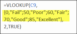
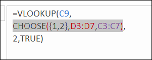
To create the table array in the VLOOKUP formula, add this CHOOSE formula:

要在VLOOKUP公式中创建表数组，请添加以下CHOOSE公式：

=VLOOKUP(C9,CHOOSE({1,2},D3:D7,C3:C7),2,TRUE)

= VLOOKUP(C9， CHOOSE( {1,2} ，D3：D7，C3：C7) ，2，TRUE)

Instead of a single index number, CHOOSE has 2 numbers, inside curly brackets.

CHOOSE在大括号内有2个数字，而不是单个索引号。

Those numbers inside the curly brackets - {1,2} - tell Excel to create a 2-column array, with Scores in column 1, and Descriptions in column 2.

大括号内的数字- {1,2} -告诉Excel创建一个2列数组，第1列为Scores，第2列为Descriptions。

CHOOSE rearranges the columns, putting the in the order that VLOOKUP needs, so you don't need to physically change the table layout.

选择重新排列列，按VLOOKUP所需的顺序排列，因此您无需实际更改表布局。

看到选择数组 (See the CHOOSE Array)

To see the array that CHOOSE creates:

要查看CHOOSE创建的数组：

• Select the cell with the VLOOKUP formula
  选择具有VLOOKUP公式的单元格
• Select the entire CHOOSE function in the formula bar
  在编辑栏中选择整个CHOOSE功能

• On your keyboard, press the F9 key, to evaluate the selected part of the formula.
  在键盘上，按F9键，以评估公式的所选部分。
• Each pair of scores/descriptions is evaluated.
  每对分数/说明都会得到评估。

IMPORTANT: When you're finished, press the Esc key, to exit the formula, without saving the changes.

重要说明 ：完成后，按Esc键 ，退出公式，而不保存更改。

VLOOKUP获取描述 (VLOOKUP Gets the Description)

The rest of the formula is just a basic VLOOKUP.

公式的其余部分只是基本的VLOOKUP。

=VLOOKUP(C9, Table Array, 2, TRUE)

= VLOOKUP( C9 ， 表数组 ， 2 ， TRUE )

For the score entered in cell C9, VLOOKUP returns the value from column 2 of the table array, using an approximate match (TRUE).

对于在单元格C9中输入的分数，VLOOKUP使用近似匹配( TRUE )返回表数组第2列中的值。

获取样本文件 (Get the Sample File)

Go to my Contextures site to download the sample file, and to see more examples for the CHOOSE Function.

转到我的Contextures网站下载示例文件，并查看CHOOSE Function的更多示例。

The zipped file is in xlsx format, and does not contain macros.

压缩文件为xlsx格式，不包含宏。

翻译自: https://contexturesblog.com/archives/2018/11/15/excel-vlookup-to-the-left/

excel vlookup