excel导入数据校验_Excel数据验证错误消息

excel导入数据校验

Do you like to use error checking in Excel, so that problem cells are flagged, or do you turn that feature off? There are options for data validation error messages too – do you use those?

您是否要在Excel中使用错误检查，以便标记问题单元格，或者您要关闭该功能？ 也有用于数据验证错误消息的选项-您是否使用这些选项？

数据验证错误消息 (Data Validation Error Messages)

If you add a drop down list on a worksheet, or any other type of data validation, you can choose which type of Error Alert messages should be shown - Stop, Warning or Information.

如果在工作表或任何其他类型的数据验证上添加下拉列表，则可以选择应显示哪种类型的错误警报消息 -停止，警告或信息。

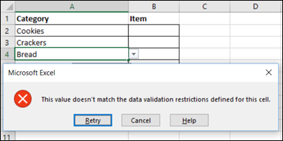
The default setting is Stop, and that prevents you from entering invalid data. An error message appears, with buttons for Retry, Cancel and Help.

默认设置为“停止”，这可以防止您输入无效的数据。 出现错误消息，其中包含用于重试，取消和帮助的按钮。

“This value doesn’t match the data validation restrictions defined for this cell.”

“此值与为此单元格定义的数据验证限制不匹配。”

响应错误消息 (Respond to the Error Message)

If you see that error message, what happens if you click one of the buttons?

如果看到该错误消息，单击按钮之一会怎样？

• Help – Takes you to a data validation page on the Microsoft website, where there are instructions for setting up a data validation cell. It won’t give you any specific details on why the value entered wasn’t valid.

  帮助 –转到Microsoft网站上的数据验证页面，其中提供了有关设置数据验证单元的说明。 它不会为您提供有关输入值为何无效的任何特定详细信息。

• Cancel – Clears the cell, so you can type a new value, or select from the drop down list, if there is one.

  取消 –清除单元格，因此您可以键入一个新值，或者如果有一个，则从下拉列表中选择。

• Retry – Highlights the value that you typed in the cell, so you can type a new value. You will have to clear the cell if you want to use the drop down arrow.

  重试 –突出显示您在单元格中键入的值，以便您可以键入新值。 如果要使用下拉箭头，则必须清除单元格。

自定义错误消息 (Customized Error Messages)

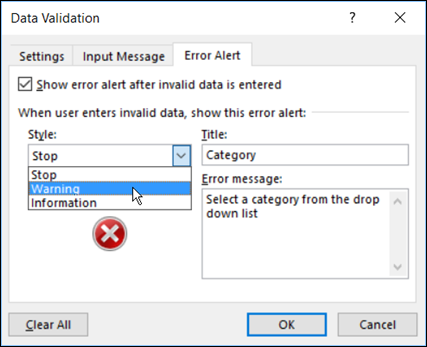
Instead of leaving the default settings for data validation errors, you can go to the Error Alert tab in the data validation dialog box, and customize them.

可以保留数据验证对话框中的“错误警报”选项卡，然后自定义它们，而不是保留数据验证错误的默认设置。

Choose one of the Styles, and enter a Title and Error message that will give people details on what went wrong.

选择一种样式，然后输入“标题和错误”消息，该消息将向人们提供发生错误的详细信息。

In this example, I selected Warning style, and entered a customized message. When I enter an item that isn’t in the list, the customized message appears, with a Warning icon, and different buttons.

在此示例中，我选择了“警告”样式，然后输入了自定义消息。 当我输入不在列表中的项目时，将显示自定义消息，警告图标和其他按钮。

关闭错误消息 (Turn Off Error Messages)

In some cases, you might want to turn off the data validation error alerts completely, like I do when allowing multiple selections from a drop down list.

在某些情况下，您可能希望完全关闭数据验证错误警报，就像在允许从下拉列表中进行多个选择时一样。

On the Error Alert tab, remove the check mark from “Show error alert after invalid data is entered”

在“错误警报”选项卡上，从“输入无效数据后显示错误警报”中删除复选标记

表中的数据验证错误消息 (Data Validation Error Messages in Tables)

If you’re using data validation in a named Excel table, invalid data might be flagged by Excel's Error Checking Rules, even if you turned off error alerts, or set the Style to Warning or Information.

如果您在命名的Excel表中使用数据验证，则即使关闭了错误警报或将“样式”设置为“警告”或“信息”，Excel的“错误检查规则”也可能会标记无效数据。

In the screen shot below, there is a warning on cell C2, because two items are in the cell.

在下面的屏幕快照中，单元格C2上有一个警告，因为该单元格中有两项。

If you copied cell C2 to a different part of the worksheet, outside of a table, the error warning would disappear – it only affects tables.

如果将单元格C2复制到工作表的不同部分(表的外部)，错误警告将消失-它仅影响表。

关闭表格数据设置 (Turn Off Table Data Setting)

If you know that there isn’t really a problem with the cell’s data, you can simply ignore the error warnings. Or, if there are just a few messages, you can set the error warning in each cell manually, to Ignore Error.

如果您知道单元格数据确实没有问题，则可以简单地忽略错误警告。 或者，如果只有几条消息，则可以在每个单元格中手动将错误警告设置为“忽略错误”。

If you want to turn off all of the data validation warnings in tables, you can follow the steps below, to change one of the Excel options.

如果要关闭表中的所有数据验证警告，可以按照以下步骤更改Excel选项之一。

• Click the arrow on the Error alert, and click Error Checking Options
  单击错误警报上的箭头，然后单击错误检查选项
• In the Options window, in the Formulas category, scroll down to the Error Checking Rules section.
  在“选项”窗口的“公式”类别中，向下滚动到“错误检查规则”部分。
• Remove the check mark for “Data entered in a table is invalid”.
  取消选中“表中输入的数据无效”的复选标记。
• Click OK.
  单击确定。

Keep in mind though, that Excel will stop flagging ALL data errors in your tables, in ALL workbooks that you open. You can read the details on my website.

但是请记住，Excel将停止标记您打开的所有工作簿中的表中的所有数据错误。 您可以在我的网站上阅读详细信息 。

视频：数据验证消息 (Video: Data Validation Messages)

To see the steps for creating a data validation input message or error message, watch this short video tutorial.

要查看创建数据验证输入消息或错误消息的步骤，请观看此简短视频教程。

演示地址

翻译自: https://contexturesblog.com/archives/2016/10/20/excel-data-validation-error-messages/

excel导入数据校验