单元格显示两个颜色_根据两个条件突出显示单元格

单元格显示两个颜色

Happy New Year! I hope you had time to relax over the holidays, and you stepped away from the computer for a while. Unless you were using the computer as excuse to hide away from all the holiday chaos! Now we’re back to work, and one of the first questions I got this year was how to highlight cells based on two conditions.

新年快乐！ 我希望您有时间在假期中放松一下，并且暂时离开计算机一段时间。 除非您使用计算机作为躲避所有假期混乱的借口！ 现在我们重新开始工作，今年我遇到的第一个问题是如何根据两个条件突出显示单元格。

使细胞变红 (Turn Cells Red)

The person who sent the question wanted to highlight cells based on 2 conditions:

发送问题的人想根据两种情况突出显示单元格：

1. The country code “US”  is entered in cell B2.
   在单元格B2中输入国家代码“ US”。
2. The data entry cell contains "United States"
   数据输入单元格包含“美国”

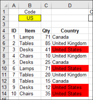
Here’s what the worksheet looks like, after that conditional formatting is set up in cells D5:D14

在单元格D5：D14中设置了条件格式后，工作表如下所示

输入2个条件 (Enter the 2 Conditions)

There isn’t a built-in conditional formatting rule that will do this. We’ll need to set up a special rule for this, using a formula.

没有内置的条件格式设置规则可以做到这一点。 我们需要使用公式为此设置一条特殊规则。

In that formula, you could hard-code the “US” and “United States” conditions. However, I like to put the conditions in worksheet cells instead, so it’s easy to see them, and change the conditions later, if you need to.

在该公式中，您可以对“ US”和“ United States”条件进行硬编码。 但是，我喜欢将条件放入工作表单元格中，因此很容易看到它们，并在以后根据需要更改条件。

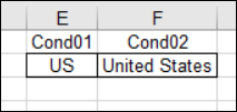
In this workbook, the conditions are in cells E2 and F2, on the same sheet as the data entry cells. You could put them on a different sheet, if you prefer, to prevent people from accidentally changing them. You could also name the cells, and use those names in the conditional formatting formula.

在此工作簿中，条件在单元格E2和F2中，与数据输入单元格在同一页上。 如果愿意，可以将它们放在另一张纸上，以防止人们意外更改它们。 您也可以命名单元格 ，并在条件格式公式中使用这些名称。

添加国家代码单元格 (Add the Country Code Cell)

People will type a country code in cell B2, so I filled that cell with yellow, to make it stand out. For testing, I put “US” in that cell.

人们将在B2单元格中输入国家/地区代码，因此我用黄色填充了该单元格，以使其突出。 为了进行测试，我将“ US”放入该单元格中。

添加条件格式 (Add the Conditional Formatting)

The next step is to add conditional formatting to the country cells in the data range  D5:D14. We’ll use the AND function, to check both conditions, and the formula is explained in the next section.

下一步是将条件格式添加到数据范围D5：D14中的国家/地区单元。 我们将使用AND函数来检查这两个条件，该公式将在下一部分中进行说明 。

• Select cells D5:D14, where the country names are listed for the orders
  选择单元格D5：D14，其中列出了订单的国家/地区名称
• On the Ribbon's Home tab, click Conditional Formatting, then click New Rule
  在功能区的“主页”选项卡上，单击“条件格式”，然后单击“新规则”。

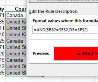
• Click Use a Formula to Determine Which Cells to Format

  单击“ 使用公式来确定要格式化的单元格”

• For the formula, enter    =AND($B$2=$E$2,D5=$F$2)

  对于公式，输入= AND($ B $ 2 = $ E $ 2，D5 = $ F $ 2)

• Click the Format button.
  单击格式按钮。
• Select red as the fill colour, and click OK
  选择红色作为填充色，然后单击“确定”。

•   Click OK, to apply the conditional formatting
  单击确定，以应用条件格式

单元格突出显示 (Cells Are Highlighted)

Because "US" is entered in cell B2, any cell in D5:D14 that contains "United States" is coloured red.

因为在单元格B2中输入了“ US”，所以D5：D14中任何包含“美国”的单元格都被涂成红色。

公式如何运作 (How the Formula Works)

The conditional formatting formula is: =AND($B$2=$E$2,D5=$F$2)

条件格式公式为： = AND($ B $ 2 = $ E $ 2，D5 = $ F $ 2)

The AND function checks the 2 conditions:

AND功能检查2种情况：

1. Does cell B2 match the condition entered in cell E2
   单元格B2是否符合在单元格E2中输入的条件
2. Does the data entry cell (D5) match the condition entered in cell F2
   数据输入单元格(D5)是否匹配在单元格F2中输入的条件

Cell D5 is used in the formula, because that was the active cell when the conditional formatting was applied.

公式中使用了单元格D5，因为在应用条件格式设置时它是活动单元格。

Some of the references are Absolute, and one is Relative:

一些引用是绝对引用，一个是相对引用：

• Absolute references are used for $B$2, $E$2 and $F$2 because no matter where the conditional formatting is applied, it should always check those cells.
  绝对引用用于$ B $ 2，$ E $ 2和$ F $ 2，因为无论在何处应用条件格式，它都应始终检查那些单元格。
• A relative reference is used for the data entry cell (D5), because it should adjust to match each cell where the conditional formatting is applied.
  相对引用用于数据输入单元格(D5)，因为它应进行调整以匹配应用条件格式的每个单元格。

获取样本文件 (Get the Sample File)

To see how this conditional formatting works, you can download the sample file. Go to the Conditional Formatting Examples page on my Contextures website. Scroll down to the Download section, and click the link to get the workbook.

若要查看此条件格式的工作方式，可以下载示例文件。 转到我的Contextures网站上的“ 条件格式示例”页面 。 向下滚动到“下载”部分，然后单击链接以获取工作簿。

The zipped file is in xlsx format (or xls format for Excel 2003), and does not contain any macros.

压缩文件为xlsx格式(对于Excel 2003，则为xls格式)，并且不包含任何宏。

翻译自: https://contexturesblog.com/archives/2017/01/05/highlight-cells-based-on-two-conditions/

单元格显示两个颜色