如何在Excel中使用VLOOKUP

VLOOKUP is one of Excel’s most useful functions, and it’s also one of the least understood.  In this article, we demystify VLOOKUP by way of a real-life example.  We’ll create a usable Invoice Template for a fictitious company.

VLOOKUP是Excel最有用的功能之一，也是了解最少的功能之一。 在本文中，我们通过一个真实的例子来揭开VLOOKUP的神秘面纱。 我们将为一个虚拟公司创建一个可用的发票模板 。

VLOOKUP is an Excel function.  This article will assume that the reader already has a passing understanding of Excel functions, and can use basic functions such as SUM, AVERAGE, and TODAY.  In its most common usage, VLOOKUP is a database function, meaning that it works with database tables – or more simply, lists of things in an Excel worksheet.  What sort of things?   Well, any sort of thing.  You may have a worksheet that contains a list of employees, or products, or customers, or CDs in your CD collection, or stars in the night sky.  It doesn’t really matter.

VLOOKUP是一个Excel 函数 。 本文将假定读者已经对Excel函数有一定的了解，并且可以使用诸如SUM，AVERAGE和TODAY之类的基本函数。 在最常见的用法中，VLOOKUP是数据库功能，这意味着它可与数据库表一起使用，或更简单地说，与Excel工作表中的事物列表一起使用。 什么样的东西 好吧， 任何事情。 您可能有一个工作表，其中包含员工，产品，客户，CD集合中的CD或夜空中的星星的列表。 没关系。

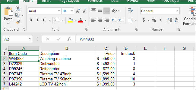
Here’s an example of a list, or database.  In this case it’s a list of products that our fictitious company sells:

这是列表或数据库的示例。 在这种情况下，这是我们的虚拟公司销售的产品清单：

Usually lists like this have some sort of unique identifier for each item in the list.  In this case, the unique identifier is in the “Item Code” column.  Note:  For the VLOOKUP function to work with a database/list, that list must have a column containing the unique identifier (or “key”, or “ID”), and that column must be the first column in the table.  Our sample database above satisfies this criterion.

通常，这样的列表对于列表中的每个项目都有某种唯一标识符。 在这种情况下，唯一标识符位于“项目代码”列中。 注意：为了使VLOOKUP函数与数据库/列表一起使用，该列表必须具有包含唯一标识符(或“键”或“ ID”)的列 ，并且该列必须是表中的第一列 。 上面的示例数据库满足了这一标准。

The hardest part of using VLOOKUP is understanding exactly what it’s for.  So let’s see if we can get that clear first:

使用VLOOKUP的最难的部分是确切地了解其用途。 因此，让我们看看是否可以先弄清楚这一点：

VLOOKUP retrieves information from a database/list based on a supplied instance of the unique identifier.

VLOOKUP基于提供的唯一标识符实例从数据库/列表中检索信息。

In the example above, you would insert the VLOOKUP function into another spreadsheet with an item code, and it would return to you either the corresponding item’s description, its price, or its availability (its “In stock” quantity) as described in your original list.  Which of these pieces of information will it pass you back?  Well, you get to decide this when you’re creating the formula.

在上面的示例中，您将VLOOKUP函数插入带有商品代码的另一个电子表格中，它将返回给您原始商品中所述的相应商品的描述，价格或可用性(“现货”数量)清单。 这些信息中的哪一条会带您回去？ 好了，您在创建公式时就可以决定这一点。

If all you need is one piece of information from the database, it would be a lot of trouble to go to to construct a formula with a VLOOKUP function in it.  Typically you would use this sort of functionality in a reusable spreadsheet, such as a template.  Each time someone enters a valid item code, the system would retrieve all the necessary information about the corresponding item.

如果您只需要数据库中的一条信息，那么在其中构造带有VLOOKUP函数的公式将很麻烦。 通常，您会在可重用的电子表格(例如模板)中使用这种功能。 每次有人输入有效的商品代码，系统都会检索有关相应商品的所有必要信息。

Let’s create an example of this:  An Invoice Template that we can reuse over and over in our fictitious company.

让我们创建一个示例：一个发票模板 ，我们可以在虚拟公司中反复使用它。

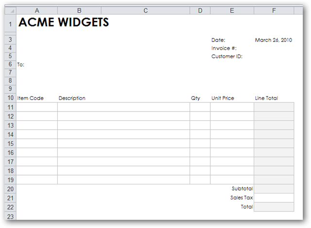
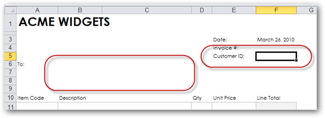
First we start Excel, and we create ourselves a blank invoice:

首先，我们启动Excel，然后为自己创建一个空白发票：

This is how it’s going to work:  The person using the invoice template will fill in a series of item codes in column “A”, and the system will retrieve each item’s description and price from our product database. That information will be used to calculate the line total for each item (assuming we enter a valid quantity).

这就是它的工作方式：使用发票模板的人员将在“ A”列中填写一系列商品代码，系统将从我们的产品数据库中检索每个商品的描述和价格。 该信息将用于计算每个项目的行总计(假设我们输入有效数量)。

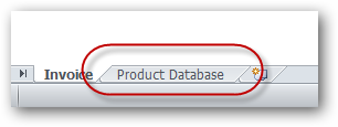
For the purposes of keeping this example simple, we will locate the product database on a separate sheet in the same workbook:

为了使该示例保持简单，我们将产品数据库放在同一工作簿的另一张纸上：

In reality, it’s more likely that the product database would be located in a separate workbook.  It makes little difference to the VLOOKUP function, which doesn’t really care if the database is located on the same sheet, a different sheet, or a completely different workbook.

实际上，产品数据库更有可能位于单独的工作簿中。 它与VLOOKUP函数没有什么区别，该函数并不真正在乎数据库是位于同一工作表，不同工作表还是完全不同的工作簿上。

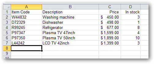
So, we’ve created our product database, which looks like this:

因此，我们创建了产品数据库，如下所示：

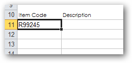
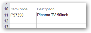
In order to test the VLOOKUP formula we’re about to write, we first enter a valid item code into cell A11 of our blank invoice:

为了测试我们将要编写的VLOOKUP公式，我们首先在空白发票的单元格A11中输入有效的商品代码：

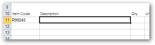
Next, we move the active cell to the cell in which we want information retrieved from the database by VLOOKUP to be stored.  Interestingly, this is the step that most people get wrong.  To explain further:  We are about to create a VLOOKUP formula that will retrieve the description that corresponds to the item code in cell A11.  Where do we want this description put when we get it?  In cell B11, of course.  So that’s where we write the VLOOKUP formula: in cell B11. Select cell B11 now.

接下来，我们将活动单元格移动到要存储通过VLOOKUP从数据库中检索到的信息的单元格中。 有趣的是，这是大多数人都会犯错的步骤。 进一步说明：我们将创建一个VLOOKUP公式，该公式将检索与单元格A11中的物料代码相对应的描述。 收到此说明后，我们希望将其放在哪里？ 当然，在单元格B11中。 这就是我们在单元格B11中编写VLOOKUP公式的地方。 现在选择单元格B11。

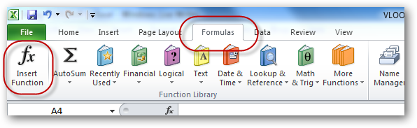
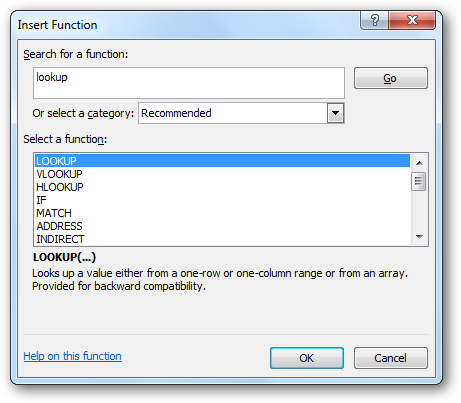
We need to locate the list of all available functions that Excel has to offer, so that we can choose VLOOKUP and get some assistance in completing the formula.  This is found by first clicking the Formulas tab, and then clicking Insert Function:

我们需要找到Excel必须提供的所有可用函数的列表，以便我们可以选择VLOOKUP并获得一些帮助来完成公式。 通过首先单击“ 公式”选项卡，然后单击“ 插入函数”可以找到它 ：

A box appears that allows us to select any of the functions available in Excel.

出现一个框，允许我们选择Excel中可用的任何功能。

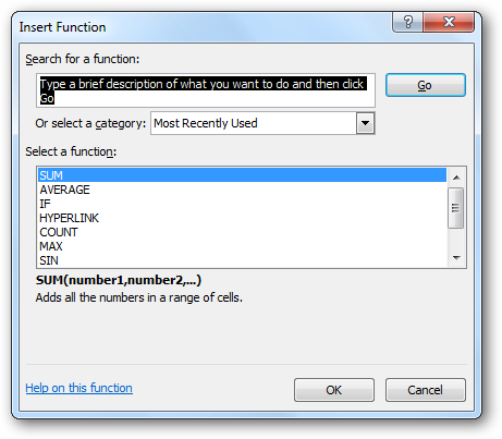
To find the one we’re looking for, we could type a search term like “lookup” (because the function we’re interested in is a lookup function).  The system would return us a list of all lookup-related functions in Excel.  VLOOKUP is the second one in the list.  Select it an click OK.

为了找到我们想要的那个，我们可以输入一个搜索词，例如“ lookup”(因为我们感兴趣的功能是一个lookup函数)。 系统将向我们返回Excel中所有与查找相关的功能的列表。 VLOOKUP是列表中的第二个。 选择它，然后单击“ 确定” 。

The Function Arguments box appears, prompting us for all the arguments (or parameters) needed in order to complete the VLOOKUP function.  You can think of this box as the function asking us the following questions:

出现“ 函数参数”框，提示我们输入完成VLOOKUP函数所需的所有参数 (或parameters )。 您可以将此框视为向我们询问以下问题的函数：

1. What unique identifier are you looking up in the database?

   您正在数据库中查找什么唯一标识符？

2. Where is the database?

   数据库在哪里？

3. Which piece of information from the database, associated with the unique identifier, do you wish to have retrieved for you?

   您希望为您检索到数据库中与唯一标识符关联的哪条信息？

The first three arguments are shown in bold, indicating that they are mandatory arguments (the VLOOKUP function is incomplete without them and will not return a valid value).  The fourth argument is not bold, meaning that it’s optional:

前三个参数以粗体显示 ，表明它们是强制性参数(没有它们，VLOOKUP函数是不完整的，并且不会返回有效值)。 第四个参数不是粗体，表示它是可选的：

We will complete the arguments in order, top to bottom.

我们将按顺序从上到下完成参数。

The first argument we need to complete is the Lookup_value argument.  The function needs us to tell it where to find the unique identifier (the item code in this case) that it should be returning the description of.  We must select the item code we entered earlier (in A11).

我们需要完成的第一个参数是Lookup_value参数。 函数需要我们告诉它在哪里可以找到唯一的标识符(在这种情况下为商品代码 )，该标识符应返回其描述。 我们必须选择我们先前输入的项目代码(在A11中)。

Click on the selector icon to the right of the first argument:

单击第一个参数右边的选择器图标：

Then click once on the cell containing the item code (A11), and press Enter:

然后，在包含商品代码(A11)的单元格上单击一次，然后按Enter ：

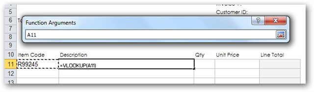
The value of “A11” is inserted into the first argument.

“ A11”的值将插入第一个参数。

Now we need to enter a value for the Table_array argument.  In other words, we need to tell VLOOKUP where to find the database/list.  Click on the selector icon next to the second argument:

现在我们需要为Table_array参数输入一个值。 换句话说，我们需要告诉VLOOKUP在哪里可以找到数据库/列表。 单击第二个参数旁边的选择器图标：

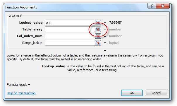
Now locate the database/list and select the entire list – not including the header line.  In our example, the database is located on a separate worksheet, so we first click on that worksheet tab:

现在，找到数据库/列表并选择整个列表- 不包括标题行 。 在我们的示例中，数据库位于单独的工作表上，因此我们首先单击该工作表选项卡：

Next we select the entire database, not including the header line:

接下来，我们选择整个数据库，不包括标题行：

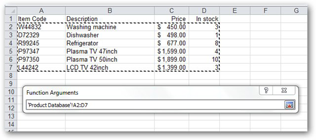
…and press Enter.  The range of cells that represents the database (in this case “’Product Database’!A2:D7”) is entered automatically for us into the second argument.

…然后按Enter 。 代表数据库的单元格范围(在本例中为“'Product Database'！A2：D7”)将自动为我们输入到第二个参数中。

Now we need to enter the third argument, Col_index_num.  We use this argument to specify to VLOOKUP which piece of information from the database, associate with our item code in A11, we wish to have returned to us.  In this particular example, we wish to have the item’s description returned to us.  If you look on the database worksheet, you’ll notice that the “Description” column is the second column in the database.  This means that we must enter a value of “2” into the Col_index_num box:

现在我们需要输入第三个参数Col_index_num 。 我们使用该参数向VLOOKUP指定来自数据库的哪些信息，并与我们在A11中的项目代码相关联，我们希望已经返回给我们。 在此特定示例中，我们希望将商品的描述返回给我们。 如果查看数据库工作表，则会注意到“描述”列是数据库中的第二列。 这意味着我们必须在Col_index_num框中输入值“ 2”：

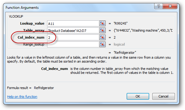
It is important to note that that we are not entering a “2” here because the “Description” column is in the B column on that worksheet.  If the database happened to start in column K of the worksheet, we would still enter a “2” in this field because the “Description” column is the second column in set of cells we selected when specifying the “Table_array”.

重要的是要注意，我们此处未输入“ 2”，因为“描述”列位于该工作表的B列中。 如果数据库恰巧从工作表的K列开始，则我们仍将在此字段中输入“ 2”，因为“ Description”列是在指定“ Table_array”时选择的单元格集中的第二列。

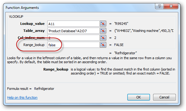
Finally, we need to decide whether to enter a value into the final VLOOKUP argument, Range_lookup.  This argument requires either a true or false value, or it should be left blank.  When using VLOOKUP with databases (as is true 90% of the time), the way to decide what to put in this argument can be thought of as follows:

最后，我们需要确定是否在最终的VLOOKUP参数Range_lookup中输入一个值。 此参数需要为true或false ，或者应为空。 当对数据库使用VLOOKUP时(实际上有90％的时间是正确的)，可以考虑以下决定在该参数中放入内容的方法：

If the first column of the database (the column that contains the unique identifiers) is sorted alphabetically/numerically in ascending order, then it’s possible to enter a value of true into this argument, or leave it blank.

如果数据库的第一列(包含唯一标识符的列)以字母/数字升序排序，则可以在此参数中输入true值，或将其保留为空白。

If the first column of the database is not sorted, or it’s sorted in descending order, then you must enter a value of false into this argument

如果数据库的第一列未排序或以降序排序，则必须在此参数中输入false值

As the first column of our database is not sorted, we enter false into this argument:

由于数据库的第一列未排序，因此在此参数中输入false ：

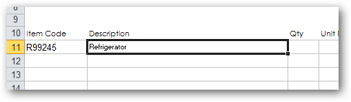
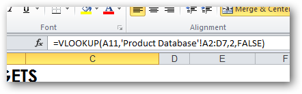
That’s it!  We’ve entered all the information required for VLOOKUP to return the value we need.  Click the OK button and notice that the description corresponding to item code “R99245” has been correctly entered into cell B11:

而已！ 我们已经输入了VLOOKUP返回所需值的所有信息。 单击“ 确定”按钮，注意与项目代码“ R99245”相对应的描述已正确输入到单元格B11中：

The formula that was created for us looks like this:

为我们创建的公式如下所示：

If we enter a different item code into cell A11, we will begin to see the power of the VLOOKUP function:  The description cell changes to match the new item code:

如果我们在单元格A11中输入其他商品代码，我们将开始看到VLOOKUP函数的功能：描述单元会更改为与新商品代码匹配：

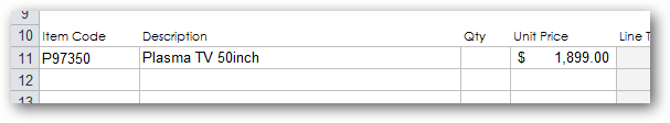
We can perform a similar set of steps to get the item’s price returned into cell E11.  Note that the new formula must be created in cell E11.  The result will look like this:

我们可以执行一组类似的步骤，以将商品的价格返回到单元格E11中。 请注意，必须在单元格E11中创建新公式。 结果将如下所示：

…and the formula will look like this:

…公式将如下所示：

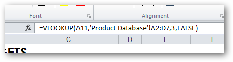
Note that the only difference between the two formulae is the third argument (Col_index_num) has changed from a “2” to a “3” (because we want data retrieved from the 3rd column in the database).

请注意，两个公式之间的唯一区别是第三个参数( Col_index_num )已从“ 2”更改为“ 3”(因为我们希望从数据库的第3列中检索数据)。

If we decided to buy 2 of these items, we would enter a “2” into cell D11.  We would then enter a simple formula into cell F11 to get the line total:

如果我们决定购买其中2件，则在单元格D11中输入“ 2”。 然后，我们将在单元格F11中输入一个简单公式以得出行总数：

=D11*E11

= D11 * E11

…which looks like this…

看起来像这样

完成发票模板 (Completing the Invoice Template)

We’ve learned a lot about VLOOKUP so far.  In fact, we’ve learned all we’re going to learn in this article.  It’s important to note that VLOOKUP can be used in other circumstances besides databases.  This is less common, and may be covered in future How-To Geek articles.

到目前为止，我们已经学到了很多有关VLOOKUP的知识。 实际上，我们已经学到了本文中要学的所有知识。 重要的是要注意，VLOOKUP可以在数据库以外的其他情况下使用。 这种情况不太常见，以后的“ How-To Geek”文章中可能会介绍。

Our invoice template is not yet complete.  In order to complete it, we would do the following:

我们的发票模板尚未完成。 为了完成它，我们将执行以下操作：

1. We would remove the sample item code from cell A11 and the “2” from cell D11.  This will cause our newly created VLOOKUP formulae to display error messages:

   我们将从单元格A11中删除示例商品代码，并从单元格D11中删除“ 2”。 这将导致我们新创建的VLOOKUP公式显示错误消息：

   

   We can remedy this by judicious use of Excel’s

   我们可以通过明智地使用Excel的

   IF() and ISBLANK() functions.  We change our formula from this…      =VLOOKUP(A11,’Product Database’!A2:D7,2,FALSE)…to this…=IF(ISBLANK(A11),””,VLOOKUP(A11,’Product Database’!A2:D7,2,FALSE))

   IF()和ISBLANK()函数。 我们将公式从此… = VLOOKUP(A11，'产品数据库'！A2：D7,2，FALSE) …更改为... = IF(ISBLANK(A11)，”“，VLOOKUP(A11，'产品数据库'！A2 ：D7,2，FALSE))

2. We would copy the formulas in cells B11, E11 and F11 down to the remainder of the item rows of the invoice.  Note that if we do this, the resulting formulas will no longer correctly refer to the database table.  We could fix this by changing the cell references for the database to absolute cell references.  Alternatively – and even better – we could create a range name for the entire product database (such as “Products”), and use this range name instead of the cell references.  The formula would change from this…      =IF(ISBLANK(A11),””,VLOOKUP(A11,’Product Database’!A2:D7,2,FALSE))…to this…      =IF(ISBLANK(A11),””,VLOOKUP(A11,Products,2,FALSE))…and then copy the formulas down to the rest of the invoice item rows.

   我们将把单元格B11，E11和F11中的公式复制到发票项目行的其余部分。 请注意，如果执行此操作，则生成的公式将不再正确引用数据库表。 我们可以通过将数据库的单元格引用更改为绝对单元格引用来解决此问题。 或者(甚至更好)，我们可以为整个产品数据库(例如“产品”)创建一个范围名称 ，并使用该范围名称代替单元格引用。 该公式将从此改变...... = IF(ISBLANK(A11)，””，VLOOKUP(A11， '产品数据库' A2：D7,2，FALSE))...这个... = IF(ISBLANK(A11)“，” ，VLOOKUP(A11，Products，2，FALSE)) … 然后将公式复制到发票项目的其余行。

3. We would probably “lock” the cells that contain our formulae (or rather unlock the other cells), and then protect the worksheet, in order to ensure that our carefully constructed formulae are not accidentally overwritten when someone comes to fill in the invoice.

   我们可能会“锁定”包含我们公式的单元格(或更确切地说，将其他单元格解锁 )，然后保护工作表，以确保当有人要填写发票时，精心构造的公式不会被意外覆盖。

4. We would save the file as a template, so that it could be reused by everyone in our company

   我们将文件另存为模板 ，以便公司中的每个人都可以重复使用

If we were feeling really clever, we would create a database of all our customers in another worksheet, and then use the customer ID entered in cell F5 to automatically fill in the customer’s name and address in cells B6, B7 and B8.

如果我们真的很聪明，可以在另一个工作表中创建一个包含所有客户的数据库，然后使用在单元格F5中输入的客户ID在B6，B7和B8单元格中自动填写客户的姓名和地址。

If you would like to practice with VLOOKUP, or simply see our resulting Invoice Template, it can be downloaded from here.

如果您想练习VLOOKUP，或者只是看到我们生成的发票模板，可以从此处下载 。

翻译自: https://www.howtogeek.com/howto/13780/using-vlookup-in-excel/