如何防止单元格在Google表格中进行编辑

Protecting individual cells in Google Sheets is a great way to prevent data in your spreadsheet from getting changed—accidentally or intentionally—by anyone viewing the sheet. Fortunately, Sheets provides a handy tool to prevents people from altering cells in your document.

保护Google表格中的各个单元格是一种很好的方法，可以防止任何查看表格的人有意或无意地更改电子表格中的数据。 幸运的是，Sheets提供了一个方便的工具来防止人们更改文档中的单元格。

保护Google表格中的单元格 (Protecting Cells in Google Sheets)

One of the best features of Google Sheets (and all the other Google apps) is the ability for anyone with edit access to collaborate on documents in the cloud. However, sometimes you don’t want the people you’re sharing a document with to edit specific cells in your sheet without completely revoking their ability to edit. This where protecting specific cells comes in handy.

Google表格(以及所有其他所有Google应用)的最佳功能之一是，具有编辑权限的任何人都可以在云中对文档进行协作。 但是，有时您不希望与文档共享的人员在不完全取消其编辑能力的情况下编辑工作表中的特定单元格。 这在保护特定细胞方面很方便。

Fire up your browser, open a Google Sheet that has cells you want to protect, and then select the cells.

启动浏览器，打开包含您要保护的单元格的Google表格，然后选择单元格。

With the cells selected, open the “Data” menu and then click “Protect Sheets and Ranges.”

选择单元格后，打开“数据”菜单，然后单击“保护图纸和范围”。

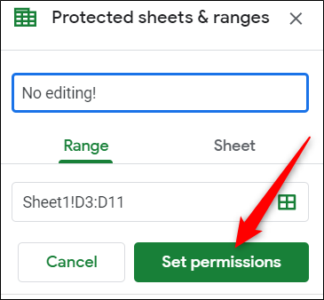
The Protected Sheets and Ranges pane appears on the right. Here, you can enter a brief description and then click “Set Permissions” to customize the cell’s protection permissions.

“保护的图纸和范围”窗格显示在右侧。 在这里，您可以输入简短说明，然后单击“设置权限”以自定义单元的保护权限。

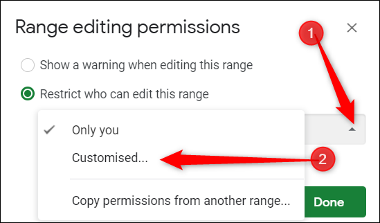
By default, anyone who already has permission to edit the document is allowed to edit every cell on the page. Click the drop-down menu under “Restrict Who Can Edit This Range” and then click “Customized” to set who is permitted to edit the selected cells.

默认情况下，任何有权编辑文档的人都可以编辑页面上的每个单元格。 单击“限制谁可以编辑此范围”下的下拉菜单，然后单击“自定义”以设置允许谁编辑所选单元格。

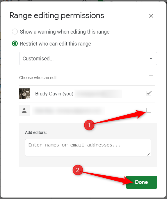
Under the list of people who can edit, everyone with whom you’ve shared edit permissions is already selected by default. Deselect anyone you don’t want to be able to edit the selected cells and then click “Done.”

在可以编辑的人员列表下，默认情况下已选择与您共享编辑权限的所有人。 取消选择您不想编辑所选单元格的任何人，然后单击“完成”。

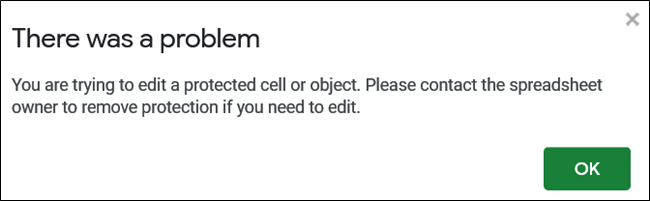
Now, anytime someone without permission to edit these cells attempts to make any changes, a prompt with the following message in Sheets comes up:

现在，任何时候未经许可编辑这些单元格的人尝试进行任何更改时，在Sheets中都会出现带有以下消息的提示：

()

编辑单元格时如何显示警告消息 (How to Show a Warning Message When Editing Cells)

If you’d rather people still be able to edit the cells, but instead have a warning message for anyone who tries to edit specific cells, you can do that as well.

如果您希望人们仍然能够编辑单元格，但是对试图编辑特定单元格的任何人都显示警告消息，您也可以这样做。

From your Sheets document, head back to Data > Protected Sheets and Ranges in the toolbar.

从表格文档中，回到工具栏中的数据>受保护的表格和范围。

Next, click the permission rule you want to alter.

接下来，单击要更改的权限规则。

Click “Set Permissions.”

点击“设置权限”。

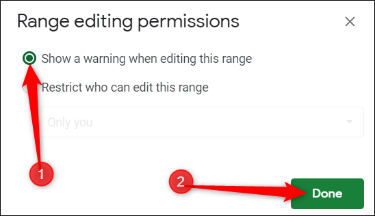
Select “Show a warning when editing this range” and then click “Done.”

选择“在编辑此范围时显示警告”，然后单击“完成”。

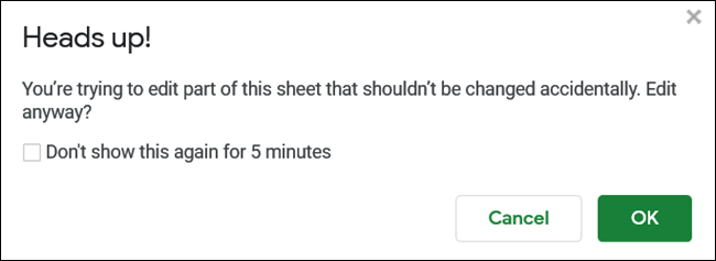
The next time anyone tries to edit any of the protected cells, they’re prompted with this message instead:

下次任何人尝试编辑任何受保护的单元格时，系统都会提示他们此消息：

保护Google表格中的整个表格 (Protecting an Entire Sheet in Google Sheets)

If you want to protect a whole sheet so that nobody except you can edit it, the easiest way is to share the sheet with them but only give them view instead of edit permission.

如果要保护整个工作表，以使除您之外的任何人都不能对其进行编辑，最简单的方法是与他们共享工作表，但只给他们查看而不是编辑权限。

However, say you wanted to protect most of a sheet, but leave a few cells open to editing— as you’d do with a form or invoice. In that case, people would still need edit permission, but it would be kind of a pain to select all the cells on the sheet except for the few on which you want to allow editing.

但是，假设您想保护工作表的大部分，但是要保留一些单元格以便编辑，就像处理表格或发票一样。 在那种情况下，人们仍然需要编辑权限，但是要选择工作表上的所有单元格(除了要允许编辑的单元格之外的单元格)会有些痛苦。

There is another way. You can protect the entire sheet and then allow access to specific cells.

还有另一种方法。 您可以保护整个工作表，然后允许访问特定的单元格。

Open up your document and head back to Data > Protected Sheets and Ranges in the toolbar.

打开文档，然后回到工具栏中的“数据”>“受保护的图纸和范围”。

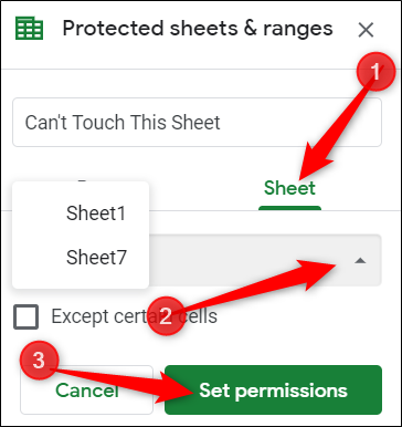
From the Protected Sheets and Ranges pane that appears on the right, click “Sheet,” choose a sheet from the drop-down menu, then click “Set Permissions.”

在右侧显示的“受保护的图纸和范围”窗格中，单击“图纸”，从下拉菜单中选择图纸，然后单击“设置权限”。

And, just like in the previous example for protecting cells, you will have to set who can edit the sheet in the window that opens up.

而且，就像前面保护单元格的示例一样，您将必须在打开的窗口中设置谁可以编辑工作表。

Click the drop-down menu under “Restrict Who Can Edit This Range,” and select “Customized” to set who is permitted to edit the selected sheet.

单击“限制谁可以编辑此范围”下的下拉菜单，然后选择“自定义”以设置允许谁编辑所选工作表。

Under the list of people who can edit, deselect anyone for whom you want to revoke edit permissions of this sheet and then click “Done.”

在可以编辑的人员列表下，取消选择要撤消此工作表的编辑权限的任何人，然后单击“完成”。

Anyone with access to your document can still open and see the contents of the sheet you’ve protected, but they aren’t able to make any changes or edits to the actual sheet.

有权访问您文档的任何人仍然可以打开并查看您保护的工作表的内容，但他们无法对实际工作表进行任何更改或编辑。

如何向受保护的工作表添加例外 (How to Add Exceptions to a Protected Sheet)

When protecting a whole sheet, Google Sheets locks every single cell. But if you want to grant edit access to only a few cells, you can specify which ones are editable.

保护整张纸时，Google表格会锁定每个单元格。 但是，如果您只想授予对少数几个单元格的编辑权限，则可以指定哪些单元格是可编辑的。

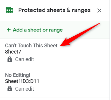
Jump back to Data > Protected Sheets and Ranges from the toolbar, then from the pane that opens, click on the protected sheet rule you want to edit.

从工具栏跳回到“数据”>“受保护的图纸和范围”，然后从打开的窗格中，单击要编辑的受保护图纸规则。

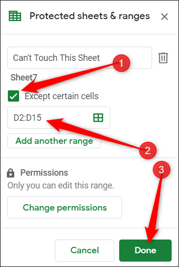
Next, toggle “Except Certain Cells” and then enter the range of cells you want to be editable. Click “Done.”

接下来，切换“除某些单元格外”，然后输入要编辑的单元格范围。 点击“完成”。

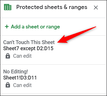
Finally, if anyone tries to edit any other cells than the ones you’ve made editable, they’ll see the same prompt as before, notifying them they can’t do that.

最后，如果有人尝试编辑除您已设置为可编辑的单元格以外的其他任何单元格，他们将看到与以前相同的提示，并通知他们无法执行此操作。

如何删除权限规则 (How to Remove Permission Rules)

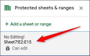
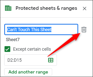
To remove any of the permission rules you just made, open up the Protected Sheets and Ranges pane by going to Data > Protected Sheets and Ranges. Once here, click the rule you want to delete.

要删除您刚刚制定的任何权限规则，请转到“数据”>“受保护的图纸和范围”，打开“受保护的图纸和范围”窗格。 在此处后，单击要删除的规则。

Next, click the trash bin, located next to the description of the rule.

接下来，单击位于规则说明旁边的垃圾桶。

You’ll be prompted to confirm that you want to remove the protected range or not. Click “Remove.”

系统将提示您确认是否要删除受保护的范围。 点击“删除”。

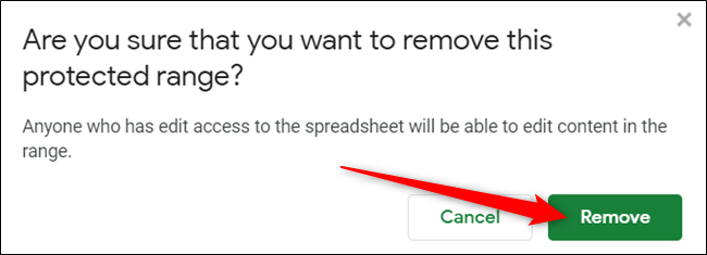
After removing the protected range, anyone who had edit access to your spreadsheet will be able to edit the content in the cells/sheets that were previously protected.

删除受保护范围后，对您的电子表格具有编辑权限的任何人都可以编辑先前受保护的单元格/工作表中的内容。

翻译自: https://www.howtogeek.com/412399/how-to-protect-cells-from-editing-in-google-sheets/