


 本文介绍了在Excel中如何冻结第一行、冻结最左边的列、自定义冻结行或列组以及同时冻结行和列的步骤,以便在浏览大型电子表格时保持关键信息如标题和标识符在视图中。

表头冻结列冻结

If you are working on a large spreadsheet, it can be useful to “freeze” certain rows or columns so that they stay on screen while you scroll through the rest of the sheet.
如果您使用的是大型电子表格,则“冻结”某些行或列以使它们在滚动表的其余部分时保留在屏幕上会很有用。
As you’re scrolling through large sheets in Excel, you might want to keep some rows or columns—like headers, for example—in view. Excel lets you freeze things in one of three ways:
当您在Excel中滚动浏览大型工作表时,您可能希望在视图中保留一些行或列(例如标题)。 Excel使您可以通过以下三种方式之一冻结内容:
- You can freeze the top row. 您可以冻结第一行。
- You can freeze the leftmost column. 您可以冻结最左边的列。
- You can freeze a pane that contains multiple rows or multiple columns—or even freeze a group of columns and a group of rows at the same time. 您可以冻结包含多行或多列的窗格,甚至可以同时冻结一组列和一组行。
So, let’s take a look at how to perform these actions.
因此,让我们看一下如何执行这些操作。
冻结第一行 (Freeze the Top Row)
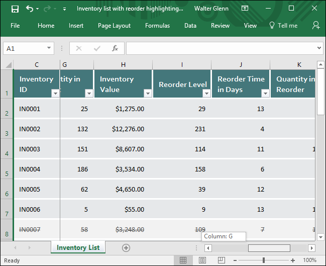
Here’s the first spreadsheet we’ll be messing with. It’s the Inventory List template that comes with Excel, in case you want to play along.
这是我们将要使用的第一个电子表格。 如果您想一起玩的话,这是Excel随附的库存清单模板。

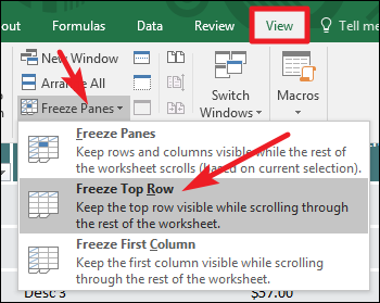
The top row in our example sheet is a header that might be nice to keep in view as you scroll down. Switch to the “View” tab, click the “Freeze Panes” dropdown menu, and then click “Freeze Top Row.”
示例表中的第一行是标题,当您向下滚动时,可以很好地保持在视图中。 切换到“查看”选项卡,单击“冻结窗格”下拉菜单,然后单击“冻结顶部行”。
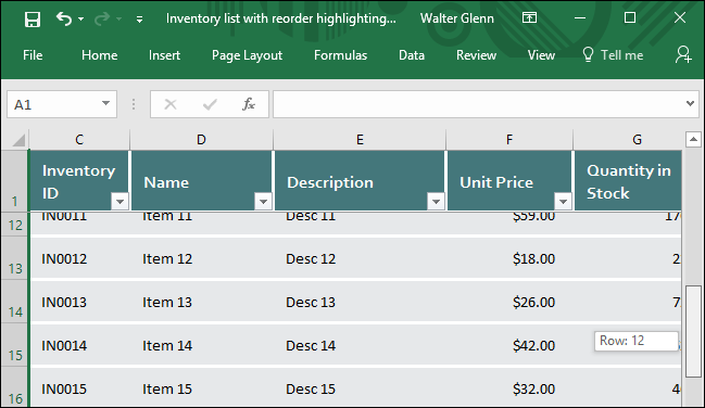
Now, when you scroll down the sheet, that top row stays in view.
现在,当您向下滚动工作表时,该第一行仍在视图中。
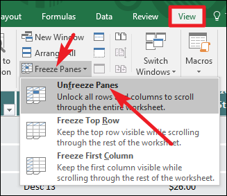
To reverse that, you just have to unfreeze the panes. On the “View” tab, hit the “Freeze Panes” dropdown again, and this time select “Unfreeze Panes.”
要扭转这种情况,您只需解冻窗格即可。 在“查看”标签上,再次点击“冻结窗格”下拉菜单,这次选择“取消冻结窗格”。
冻结左行 (Freeze the Left Row)
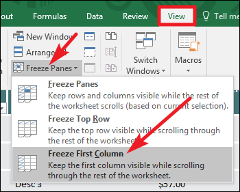
Sometimes, the leftmost column contains the information you’ll want to keep on screen as you scroll to the right on your sheet. To do that, switch to the “View” tab, click the “Freeze Panes” dropdown menu, and then click “Freeze First Column.”
有时,最左侧的列包含您在滚动到工作表的右侧时想要保留在屏幕上的信息。 为此,请切换到“查看”选项卡,单击“冻结窗格”下拉菜单,然后单击“冻结第一列”。
Now, as you scroll to the right, that first column stays on screen. In our example, it lets us keep the inventory ID column visible while we scroll through the other columns of data.
现在,当您向右滚动时,第一列将保留在屏幕上。 在我们的示例中,它使我们可以在滚动其他数据列的同时使库存ID列保持可见。
And again, to unfreeze the column, just head to View > Freeze Panes > Unfreeze Panes.
再次,要取消冻结列,只需转到“视图”>“冻结窗格”>“取消冻结窗格”。
冻结自己的行或列组 (Freeze Your Own Group of Rows or Columns)
Sometimes, the information you need to freeze on screen isn’t in the top row or first column. In this case, you’ll need to freeze a group of rows or columns. As an example, take a look at the spreadsheet below. This one is the Employee Attendance template included with Excel, if you want to load it up.
有时,您需要在屏幕上冻结的信息不在第一行或第一列中。 在这种情况下,您需要冻结一组行或列。 例如,请看下面的电子表格。 如果要加载该模板,它就是Excel随附的“员工出勤”模板。
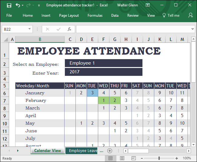
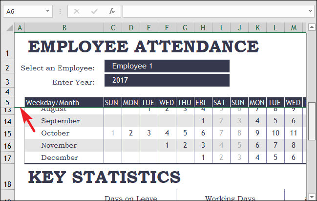
Notice that there are a bunch of rows at the top before the actual header we might want to freeze—the row with the days of the week listed. Obviously, freezing just the top row won’t work this time, so we’ll need to freeze a group of rows at the top.
请注意,在我们可能想冻结的实际标头之前,在顶部有一堆行,其中列出了星期几。 显然,这次仅冻结最上面的行是行不通的,因此我们需要冻结最上面的一组行。
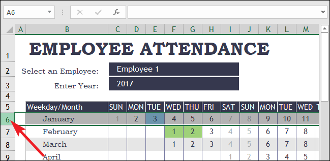
First, select the entire row below the bottom most row that you want to stay on screen. In our example, we want row five to stay on screen, so we’re selecting row six. To select the row, just click the number to the left of the row.
首先,选择要保留在屏幕最底端一行下方的整行。 在我们的示例中,我们希望第五行保留在屏幕上,因此我们选择第六行。 要选择该行,只需单击该行左侧的数字。
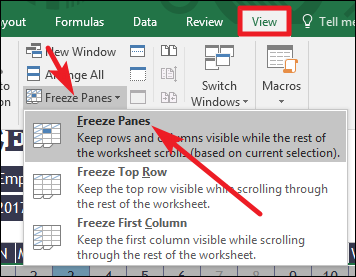
Next, switch to the “View” tab, click the “Freeze Panes” dropdown menu, and then click “Freeze Panes.”
接下来,切换到“查看”选项卡,单击“冻结窗格”下拉菜单,然后单击“冻结窗格”。
Now, as you scroll down the sheet, rows one through five are frozen. Note that a thick gray line will always show you where the freeze point is.
现在,当您向下滚动表格时,冻结第一到第五行。 请注意,粗灰线将始终显示冻结点在哪里。
To freeze a pane of columns instead, just select the whole row to the right of the right most row you want to freeze. Here, we’re selecting Row C because we want Row B to stay on screen.
要冻结列窗格,只需选择要冻结的最右边行右边的整行。 在这里,我们选择C行是因为我们希望B行停留在屏幕上。
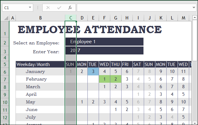
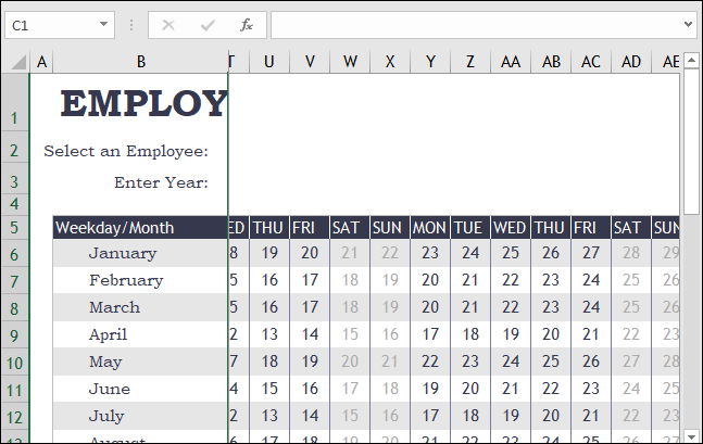
And then head to View > Freeze Panes > Freeze Panes. Now, our column showing the months stays on screen as we scroll right.
然后转到视图>冻结窗格>冻结窗格。 现在,当我们向右滚动时,显示月份的列将保留在屏幕上。
And remember, when you have frozen rows or columns and need to return to a normal view, just go to View > Freeze Panes > Unfreeze Panes.
记住,当冻结行或列并需要返回到普通视图时,只需转到视图>冻结窗格>取消冻结窗格。
同时冻结列和行 (Freeze Columns and Rows at the Same Time)
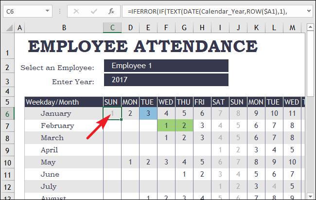
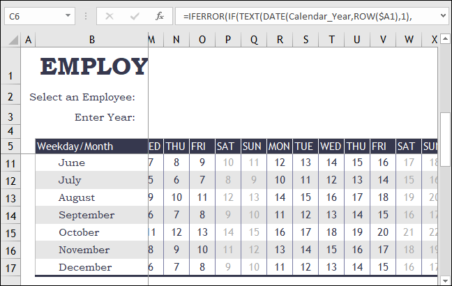
We have one more trick to show you. You’ve seen how to freeze a group of rows or a group of columns. You can also freeze rows and columns at the same time. Looking at Employee Attendance spreadsheet again, let’s say we wanted to keep both the header with the weekdays (row five) and the column with the months (column B) on screen at the same time.
我们还有另一个技巧可以向您展示。 您已经了解了如何冻结一组行或一组列。 您还可以同时冻结行和列。 再次查看“员工出勤”电子表格,假设我们希望同时在屏幕上同时保留标头和工作日(第5行)以及列和月份(B列)。
To do this, select the uppermost and leftmost cell that you don’t want to freeze. Here, we want to freeze row five and column B, so we’ll select cell C6 by clicking it.
要做到这一点,选择最上和你不想冻结左边的单元格。 在这里,我们要冻结第五行和B列,因此我们将通过单击选择单元格C6。
Next, switch to the “View” tab, click the “Freeze Panes” dropdown menu, and then click “Freeze Panes.”
接下来,切换到“查看”选项卡,单击“冻结窗格”下拉菜单,然后单击“冻结窗格”。

And now, we can scroll down or right while keeping those header rows and columns on screen.
现在,我们可以向下或向右滚动,同时在屏幕上保留这些标题行和列。
Freezing rows or columns in Excel isn’t difficult, once you know the option is there. And it can really help when navigating large, complicated spreadsheets.
知道存在该选项后,在Excel中冻结行或列并不困难。 当浏览大型,复杂的电子表格时,它确实可以提供帮助。
翻译自: https://www.howtogeek.com/166326/how-to-freeze-and-unfreeze-rows-and-columns-in-excel-2013/
表头冻结列冻结


 2361
2361

 被折叠的 条评论
为什么被折叠?
被折叠的 条评论
为什么被折叠?
 到【灌水乐园】发言


