


 Scikit-Learn是Python中最强大的机器学习库,提供丰富的工具进行分类、回归、聚类和降维等任务。它基于NumPy、SciPy和Matplotlib构建,具有高效的接口。Scikit-Learn起源于2007年的Google Summer of Code项目,由多个核心贡献者不断维护和更新。该库允许用户通过简单的API进行复杂的机器学习操作,包括PCA、增量PCA、内核PCA等降维技术。
scikit-learn
Scikit Learn-快速指南 (Scikit Learn - Quick Guide)
Scikit Learn-简介 (Scikit Learn - Introduction)
In this chapter, we will understand what is Scikit-Learn or Sklearn, origin of Scikit-Learn and some other related topics such as communities and contributors responsible for development and maintenance of Scikit-Learn, its prerequisites, installation and its features.
在本章中,我们将了解什么是Scikit-Learn或Sklearn,Scikit-Learn的起源以及其他一些相关主题,例如负责Scikit-Learn的开发和维护的社区和贡献者,其先决条件,安装及其功能。
什么是Scikit-Learn(Sklearn) (What is Scikit-Learn (Sklearn))
Scikit-learn (Sklearn) is the most useful and robust library for machine learning in Python. It provides a selection of efficient tools for machine learning and statistical modeling including classification, regression, clustering and dimensionality reduction via a consistence interface in Python. This library, which is largely written in Python, is built upon NumPy, SciPy and Matplotlib.
Scikit-learn(Sklearn)是用于Python中机器学习的最有用和最强大的库。 它通过Python中的一致性接口为机器学习和统计建模提供了一系列有效的工具,包括分类,回归,聚类和降维。 该库主要用Python编写,基于NumPy,SciPy和Matplotlib构建 。
Scikit-Learn的起源 (Origin of Scikit-Learn)
It was originally called scikits.learn and was initially developed by David Cournapeau as a Google summer of code project in 2007. Later, in 2010, Fabian Pedregosa, Gael Varoquaux, Alexandre Gramfort, and Vincent Michel, from FIRCA (French Institute for Research in Computer Science and Automation), took this project at another level and made the first public release (v0.1 beta) on 1st Feb. 2010.
它最初称为scikits.learn ,最初由David Cournapeau于2007年在Google的夏季代码项目中开发。后来,在2010年,FIRCA(法国研究学院)的Fabian Pedregosa,Gael Varoquaux,Alexandre Gramfort和Vincent Michel计算机科学与自动化),将这个项目带入了另一个层次,并于2010年2月1日发布了第一个公开版本(v0.1 beta)。
Let’s have a look at its version history −
让我们看看它的版本历史-
May 2019: scikit-learn 0.21.0
2019年5月:scikit-learn 0.21.0
March 2019: scikit-learn 0.20.3
2019年3月:scikit-learn 0.20.3
December 2018: scikit-learn 0.20.2
2018年12月:scikit-learn 0.20.2
November 2018: scikit-learn 0.20.1
2018年11月:scikit-learn 0.20.1
September 2018: scikit-learn 0.20.0
2018年9月:scikit-learn 0.20.0
July 2018: scikit-learn 0.19.2
2018年7月:scikit-learn 0.19.2
July 2017: scikit-learn 0.19.0
2017年7月:scikit-learn 0.19.0
September 2016. scikit-learn 0.18.0
2016年9月。scikit-learn 0.18.0
November 2015. scikit-learn 0.17.0
2015年11月。scikit-learn 0.17.0
March 2015. scikit-learn 0.16.0
2015年3月。scikit-learn 0.16.0
July 2014. scikit-learn 0.15.0
2014年7月。scikit-learn 0.15.0
August 2013. scikit-learn 0.14
2013年8月。scikit-learn 0.14
社区和贡献者 (Community & contributors)
Scikit-learn is a community effort and anyone can contribute to it. This project is hosted on https://github.com/scikit-learn/scikit-learn. Following people are currently the core contributors to Sklearn’s development and maintenance −
Scikit-learn是一项社区活动,任何人都可以为此做出贡献。 该项目托管在https://github.com/scikit-learn/scikit-learn上。 目前,以下人员是Sklearn开发和维护的主要贡献者-
Joris Van den Bossche (Data Scientist)
Joris Van den Bossche(数据科学家)
Thomas J Fan (Software Developer)
Thomas J Fan(软件开发人员)
Alexandre Gramfort (Machine Learning Researcher)
Alexandre Gramfort(机器学习研究员)
Olivier Grisel (Machine Learning Expert)
Olivier Grisel(机器学习专家)
Nicolas Hug (Associate Research Scientist)
Nicolas Hug(副研究员)
Andreas Mueller (Machine Learning Scientist)
Andreas Mueller(机器学习科学家)
Hanmin Qin (Software Engineer)
秦汉民(软件工程师)
Adrin Jalali (Open Source Developer)
Adrin Jalali(开源开发人员)
Nelle Varoquaux (Data Science Researcher)
Nelle Varoquaux(数据科学研究员)
Roman Yurchak (Data Scientist)
Roman Yurchak(数据科学家)
Various organisations like Booking.com, JP Morgan, Evernote, Inria, AWeber, Spotify and many more are using Sklearn.
像Booking.com,JP Morgan,Evernote,Inria,AWeber,Spotify等各种组织都在使用Sklearn。
先决条件 (Prerequisites)
Before we start using scikit-learn latest release, we require the following −
在开始使用scikit-learn最新版本之前,我们需要满足以下条件-
Python (>=3.5)
Python(> = 3.5)
NumPy (>= 1.11.0)
NumPy(> = 1.11.0)
Scipy (>= 0.17.0)li
西皮(> = 0.17.0)li
Joblib (>= 0.11)
Joblib(> = 0.11)
Matplotlib (>= 1.5.1) is required for Sklearn plotting capabilities.
Sklearn绘图功能需要Matplotlib(> = 1.5.1)。
Pandas (>= 0.18.0) is required for some of the scikit-learn examples using data structure and analysis.
使用数据结构和分析的某些scikit学习示例需要使用Pandas(> = 0.18.0)。
安装 (Installation)
If you already installed NumPy and Scipy, following are the two easiest ways to install scikit-learn −
如果您已经安装了NumPy和Scipy,则以下是安装scikit-learn的两种最简单的方法-
使用点 (Using pip)
Following command can be used to install scikit-learn via pip −
以下命令可用于通过pip安装scikit-learn-
pip install -U scikit-learn
使用conda (Using conda)
Following command can be used to install scikit-learn via conda −
以下命令可用于通过conda安装scikit-learn-
conda install scikit-learn
On the other hand, if NumPy and Scipy is not yet installed on your Python workstation then, you can install them by using either pip or conda.
另一方面,如果Python工作站上尚未安装NumPy和Scipy,则可以使用pip或conda进行安装 。
Another option to use scikit-learn is to use Python distributions like Canopy and Anaconda because they both ship the latest version of scikit-learn.
使用scikit-learn的另一种方法是使用Canopy和Anaconda之类的Python发行版,因为它们都提供了最新版本的scikit-learn。
特征 (Features)
Rather than focusing on loading, manipulating and summarising data, Scikit-learn library is focused on modeling the data. Some of the most popular groups of models provided by Sklearn are as follows −
Scikit-learn库不是专注于加载,处理和汇总数据,而是专注于对数据建模。 Sklearn提供的一些最受欢迎的模型组如下-
Supervised Learning algorithms − Almost all the popular supervised learning algorithms, like Linear Regression, Support Vector Machine (SVM), Decision Tree etc., are the part of scikit-learn.
监督学习算法 -几乎所有流行的监督学习算法,例如线性回归,支持向量机(SVM),决策树等,都是scikit-learn的一部分。
Unsupervised Learning algorithms − On the other hand, it also has all the popular unsupervised learning algorithms from clustering, factor analysis, PCA (Principal Component Analysis) to unsupervised neural networks.
无监督学习算法 -另一方面,它也具有从聚类,因子分析,PCA(主成分分析)到无监督神经网络的所有流行的无监督学习算法。
Clustering − This model is used for grouping unlabeled data.
群集 -此模型用于对未标记的数据进行分组。
Cross Validation − It is used to check the accuracy of supervised models on unseen data.
交叉验证 -用于检查看不见的数据上监督模型的准确性。
Dimensionality Reduction − It is used for reducing the number of attributes in data which can be further used for summarisation, visualisation and feature selection.
降维 -用于减少数据中的属性数量,这些属性可进一步用于汇总,可视化和特征选择。
Ensemble methods − As name suggest, it is used for combining the predictions of multiple supervised models.
集成方法 -顾名思义,它用于组合多个监督模型的预测。
Feature extraction − It is used to extract the features from data to define the attributes in image and text data.
特征提取 -用于从数据中提取特征,以定义图像和文本数据中的属性。
Feature selection − It is used to identify useful attributes to create supervised models.
特征选择 -用于识别有用的属性以创建监督模型。
Open Source − It is open source library and also commercially usable under BSD license.
开源 -它是开源库,并且在BSD许可下也可以商业使用。
Scikit学习-建模过程 (Scikit Learn - Modelling Process)
This chapter deals with the modelling process involved in Sklearn. Let us understand about the same in detail and begin with dataset loading.
本章介绍Sklearn中涉及的建模过程。 让我们详细了解一下,并从数据集加载开始。
数据集加载 (Dataset Loading)
A collection of data is called dataset. It is having the following two components −
数据的集合称为数据集。 它具有以下两个组成部分-
Features − The variables of data are called its features. They are also known as predictors, inputs or attributes.
特征 -数据的变量称为其特征。 它们也称为预测变量,输入或属性。
Feature matrix − It is the collection of features, in case there are more than one.
特征矩阵 -如果有多个特征,它是特征的集合。
Feature Names − It is the list of all the names of the features.
功能名称 -这是所有功能名称的列表。
Response − It is the output variable that basically depends upon the feature variables. They are also known as target, label or output.
响应 -基本取决于特征变量的是输出变量。 它们也称为目标,标签或输出。
Response Vector − It is used to represent response column. Generally, we have just one response column.
响应向量 -用于表示响应列。 通常,我们只有一个响应列。
Target Names − It represent the possible values taken by a response vector.
目标名称 -它表示响应向量可能采用的值。
Scikit-learn have few example datasets like iris and digits for classification and the Boston house prices for regression.
Scikit-learn几乎没有示例数据集,例如用于分类的虹膜和数字 ,以及用于回归的波士顿房价 。
例 (Example)
Following is an example to load iris dataset −
以下是加载虹膜数据集的示例-
from sklearn.datasets import load_iris
iris = load_iris()
X = iris.data
y = iris.target
feature_names = iris.feature_names
target_names = iris.target_names
print("Feature names:", feature_names)
print("Target names:", target_names)
print("\nFirst 10 rows of X:\n", X[:10])
输出量 (Output)
Feature names: ['sepal length (cm)', 'sepal width (cm)', 'petal length (cm)', 'petal width (cm)']
Target names: ['setosa' 'versicolor' 'virginica']
First 10 rows of X:
[
   [5.1 3.5 1.4 0.2]
   [4.9 3. 1.4 0.2]
   [4.7 3.2 1.3 0.2]
   [4.6 3.1 1.5 0.2]
   [5. 3.6 1.4 0.2]
   [5.4 3.9 1.7 0.4]
   [4.6 3.4 1.4 0.3]
   [5. 3.4 1.5 0.2]
   [4.4 2.9 1.4 0.2]
   [4.9 3.1 1.5 0.1]
]
分割数据集 (Splitting the dataset)
To check the accuracy of our model, we can split the dataset into two pieces-a training set and a testing set. Use the training set to train the model and testing set to test the model. After that, we can evaluate how well our model did.
为了检查模型的准确性,我们可以将数据集分为两部分:训练集和测试集 。 使用训练集训练模型,并使用测试集测试模型。 之后,我们可以评估模型的效果。
例 (Example)
The following example will split the data into 70:30 ratio, i.e. 70% data will be used as training data and 30% will be used as testing data. The dataset is iris dataset as in above example.
以下示例将数据分成70:30的比例,即70%的数据将用作训练数据,而30%的数据将用作测试数据。 数据集是虹膜数据集,如上例所示。
from sklearn.datasets import load_iris
iris = load_iris()

X = iris.data
y = iris.target

from sklearn.model_selection import train_test_split

X_train, X_test, y_train, y_test = train_test_split(
   X, y, test_size = 0.3, random_state = 1
)

print(X_train.shape)
print(X_test.shape)

print(y_train.shape)
print(y_test.shape)
输出量 (Output)
(105, 4)
(45, 4)
(105,)
(45,)
As seen in the example above, it uses train_test_split() function of scikit-learn to split the dataset. This function has the following arguments −
如上例所示,它使用scikit-learn的train_test_split()函数来拆分数据集。 此函数具有以下参数-
X, y − Here, X is the feature matrix and y is the response vector, which need to be split.
X,y-在这里, X是特征矩阵 ,y是响应向量 ,需要进行拆分。
test_size − This represents the ratio of test data to the total given data. As in the above example, we are setting test_data = 0.3 for 150 rows of X. It will produce test data of 150*0.3 = 45 rows.
test_size-这表示测试数据与总给定数据的比率。 如上例所示,我们为150行X设置了test_data = 0.3 。它将产生150 * 0.3 = 45行的测试数据。
random_size − It is used to guarantee that the split will always be the same. This is useful in the situations where you want reproducible results.
random_size-用于确保拆分将始终相同。 在需要可重现结果的情况下,这很有用。
训练模型 (Train the Model)
Next, we can use our dataset to train some prediction-model. As discussed, scikit-learn has wide range of Machine Learning (ML) algorithms which have a consistent interface for fitting, predicting accuracy, recall etc.
接下来,我们可以使用我们的数据集来训练一些预测模型。 正如讨论的那样,scikit-learn具有广泛的机器学习(ML)算法 ,这些算法具有一致的接口,可以进行拟合,预测准确性,召回率等。
例 (Example)
In the example below, we are going to use KNN (K nearest neighbors) classifier. Don’t go into the details of KNN algorithms, as there will be a separate chapter for that. This example is used to make you understand the implementation part only.
在下面的示例中,我们将使用KNN(K个最近邻居)分类器。 无需赘述KNN算法的细节,因为将有单独的章节。 本示例仅用于使您理解实现部分。
from sklearn.datasets import load_iris
iris = load_iris()
X = iris.data
y = iris.target
from sklearn.model_selection import train_test_split
X_train, X_test, y_train, y_test = train_test_split(
   X, y, test_size = 0.4, random_state=1
)
from sklearn.neighbors import KNeighborsClassifier
from sklearn import metrics
classifier_knn = KNeighborsClassifier(n_neighbors = 3)
classifier_knn.fit(X_train, y_train)
y_pred = classifier_knn.predict(X_test)
# Finding accuracy by comparing actual response values(y_test)with predicted response value(y_pred)
print("Accuracy:", metrics.accuracy_score(y_test, y_pred))
# Providing sample data and the model will make prediction out of that data

sample = [[5, 5, 3, 2], [2, 4, 3, 5]]
preds = classifier_knn.predict(sample)
pred_species = [iris.target_names[p] for p in preds] print("Predictions:", pred_species)
输出量 (Output)
Accuracy: 0.9833333333333333
Predictions: ['versicolor', 'virginica']
模型持久性 (Model Persistence)
Once you train the model, it is desirable that the model should be persist for future use so that we do not need to retrain it again and again. It can be done with the help of dump and load features of joblib package.
训练完模型后,最好保留模型以备将来使用,这样我们就不必一次又一次地重新训练它。 可以借助joblib软件包的转储和加载功能来完成 。
Consider the example below in which we will be saving the above trained model (classifier_knn) for future use −
考虑下面的示例,在该示例中,我们将保存以上训练的模型(classifier_knn)供以后使用-
from sklearn.externals import joblib
joblib.dump(classifier_knn, 'iris_classifier_knn.joblib')
The above code will save the model into file named iris_classifier_knn.joblib. Now, the object can be reloaded from the file with the help of following code −
上面的代码会将模型保存到名为iris_classifier_knn.joblib的文件中。 现在,可以在以下代码的帮助下从文件中重新加载对象:
joblib.load('iris_classifier_knn.joblib')
预处理数据 (Preprocessing the Data)
As we are dealing with lots of data and that data is in raw form, before inputting that data to machine learning algorithms, we need to convert it into meaningful data. This process is called preprocessing the data. Scikit-learn has package named preprocessing for this purpose. The preprocessing package has the following techniques −
由于我们要处理大量数据,并且这些数据是原始格式,因此在将该数据输入到机器学习算法之前,我们需要将其转换为有意义的数据。 此过程称为预处理数据。 为此,Scikit-learn具有名为预处理的软件包。 预处理程序包具有以下技术-
二值化 (Binarisation)
This preprocessing technique is used when we need to convert our numerical values into Boolean values.
当我们需要将数值转换为布尔值时,可以使用这种预处理技术。
例 (Example)
import numpy as np
from sklearn import preprocessing
Input_data = np.array(
   [2.1, -1.9, 5.5],
   [-1.5, 2.4, 3.5],
   [0.5, -7.9, 5.6],
   [5.9, 2.3, -5.8]]
)
data_binarized = preprocessing.Binarizer(threshold=0.5).transform(input_data)
print("\nBinarized data:\n", data_binarized)
In the above example, we used threshold value = 0.5 and that is why, all the values above 0.5 would be converted to 1, and all the values below 0.5 would be converted to 0.
在上面的示例中,我们使用阈值 = 0.5,这就是为什么将所有大于0.5的值都转换为1,而将所有小于0.5的值都转换为0的原因。
输出量 (Output)
Binarized data:
[
   [ 1. 0. 1.]
   [ 0. 1. 1.]
   [ 0. 0. 1.]
   [ 1. 1. 0.]
]
均值去除 (Mean Removal)
This technique is used to eliminate the mean from feature vector so that every feature centered on zero.
该技术用于消除特征向量的均值,以便每个特征都以零为中心。
例 (Example)
import numpy as np
from sklearn import preprocessing
Input_data = np.array(
   [2.1, -1.9, 5.5],
   [-1.5, 2.4, 3.5],
   [0.5, -7.9, 5.6],
   [5.9, 2.3, -5.8]]
)

#displaying the mean and the standard deviation of the input data
print("Mean =", input_data.mean(axis=0))
print("Stddeviation = ", input_data.std(axis=0))
#Removing the mean and the standard deviation of the input data

data_scaled = preprocessing.scale(input_data)
print("Mean_removed =", data_scaled.mean(axis=0))
print("Stddeviation_removed =", data_scaled.std(axis=0))
输出量 (Output)
Mean = [ 1.75 -1.275 2.2 ]
Stddeviation = [ 2.71431391 4.20022321 4.69414529]
Mean_removed = [ 1.11022302e-16 0.00000000e+00 0.00000000e+00]
Stddeviation_removed = [ 1. 1. 1.]
缩放比例 (Scaling)
We use this preprocessing technique for scaling the feature vectors. Scaling of feature vectors is important, because the features should not be synthetically large or small.
我们使用这种预处理技术来缩放特征向量。 特征向量的缩放很重要,因为特征不应该合成的大或小。
例 (Example)
import numpy as np
from sklearn import preprocessing
Input_data = np.array(
   [
      [2.1, -1.9, 5.5],
      [-1.5, 2.4, 3.5],
      [0.5, -7.9, 5.6],
      [5.9, 2.3, -5.8]
   ]
)
data_scaler_minmax = preprocessing.MinMaxScaler(feature_range=(0,1))
data_scaled_minmax = data_scaler_minmax.fit_transform(input_data)
print ("\nMin max scaled data:\n", data_scaled_minmax)
输出量 (Output)
Min max scaled data:
[
   [ 0.48648649 0.58252427 0.99122807]
   [ 0. 1. 0.81578947]
   [ 0.27027027 0. 1. ]
   [ 1. 0.99029126 0. ]
]
正常化 (Normalisation)
We use this preprocessing technique for modifying the feature vectors. Normalisation of feature vectors is necessary so that the feature vectors can be measured at common scale. There are two types of normalisation as follows −
我们使用这种预处理技术来修改特征向量。 特征向量的归一化是必要的,以便可以在公共尺度上测量特征向量。 标准化有以下两种类型-
L1归一化 (L1 Normalisation)
It is also called Least Absolute Deviations. It modifies the value in such a manner that the sum of the absolute values remains always up to 1 in each row. Following example shows the implementation of L1 normalisation on input data.
也称为最小绝对偏差。 它以使绝对值的总和在每一行中始终保持最大为1的方式修改值。 以下示例显示了对输入数据进行L1标准化的实现。
例 (Example)
import numpy as np
from sklearn import preprocessing
Input_data = np.array(
   [
      [2.1, -1.9, 5.5],
      [-1.5, 2.4, 3.5],
      [0.5, -7.9, 5.6],
      [5.9, 2.3, -5.8]
   ]
)
data_normalized_l1 = preprocessing.normalize(input_data, norm='l1')
print("\nL1 normalized data:\n", data_normalized_l1)
输出量 (Output)
L1 normalized data:
[
   [ 0.22105263 -0.2 0.57894737]
   [-0.2027027 0.32432432 0.47297297]
   [ 0.03571429 -0.56428571 0.4 ]
   [ 0.42142857 0.16428571 -0.41428571]
]
L2归一化 (L2 Normalisation)
Also called Least Squares. It modifies the value in such a manner that the sum of the squares remains always up to 1 in each row. Following example shows the implementation of L2 normalisation on input data.
也称为最小二乘。 它以这样的方式修改值,使得平方和在每一行中始终保持最大为1。 以下示例显示了对输入数据进行L2标准化的实现。
例 (Example)
import numpy as np
from sklearn import preprocessing
Input_data = np.array(
   [
      [2.1, -1.9, 5.5],
      [-1.5, 2.4, 3.5],
      [0.5, -7.9, 5.6],
      [5.9, 2.3, -5.8]
   ]
)
data_normalized_l2 = preprocessing.normalize(input_data, norm='l2')
print("\nL1 normalized data:\n", data_normalized_l2)
输出量 (Output)
L2 normalized data:
[
   [ 0.33946114 -0.30713151 0.88906489]
   [-0.33325106 0.53320169 0.7775858 ]
   [ 0.05156558 -0.81473612 0.57753446]
   [ 0.68706914 0.26784051 -0.6754239 ]
]
Scikit学习-数据表示 (Scikit Learn - Data Representation)
As we know that machine learning is about to create model from data. For this purpose, computer must understand the data first. Next, we are going to discuss various ways to represent the data in order to be understood by computer −
众所周知,机器学习即将根据数据创建模型。 为此,计算机必须首先了解数据。 接下来,我们将讨论表示数据的各种方式,以便计算机可以理解-
数据如表 (Data as table)
The best way to represent data in Scikit-learn is in the form of tables. A table represents a 2-D grid of data where rows represent the individual elements of the dataset and the columns represents the quantities related to those individual elements.
在Scikit学习中表示数据的最佳方法是表格。 表格表示数据的二维网格,其中行表示数据集的各个元素,列表示与这些单个元素相关的数量。
例 (Example)
With the example given below, we can download iris dataset in the form of a Pandas DataFrame with the help of python seaborn library.
通过下面给出的示例,我们可以借助python seaborn库以Pandas DataFrame的形式下载虹膜数据集 。
import seaborn as sns
iris = sns.load_dataset('iris')
iris.head()
输出量 (Output)
sepal_length sepal_width petal_length petal_width  species
0        5.1      3.5         1.4             0.2   setosa
1        4.9      3.0         1.4             0.2   setosa
2        4.7      3.2         1.3             0.2   setosa
3        4.6      3.1         1.5             0.2   setosa
4        5.0      3.6         1.4             0.2   setosa
From above output, we can see that each row of the data represents a single observed flower and the number of rows represents the total number of flowers in the dataset. Generally, we refer the rows of the matrix as samples.
从上面的输出中,我们可以看到数据的每一行代表一个观察到的花朵,行数代表数据集中的花朵总数。 通常,我们将矩阵的行称为样本。
On the other hand, each column of the data represents a quantitative information describing each sample. Generally, we refer the columns of the matrix as features.
另一方面,数据的每一列代表描述每个样品的定量信息。 通常,我们将矩阵的列称为要素。
数据作为特征矩阵 (Data as Feature Matrix)
Features matrix may be defined as the table layout where information can be thought of as a 2-D matrix. It is stored in a variable named X and assumed to be two dimensional with shape [n_samples, n_features]. Mostly, it is contained in a NumPy array or a Pandas DataFrame. As told earlier, the samples always represent the individual objects described by the dataset and the features represents the distinct observations that describe each sample in a quantitative manner.
特征矩阵可以定义为表格布局,其中信息可以被认为是二维矩阵。 它存储在名为X的变量中,并假定是二维的,形状为[n_samples,n_features]。 通常,它包含在NumPy数组或Pandas DataFrame中。 如前所述,样本始终代表数据集描述的单个对象,而要素代表以定量方式描述每个样本的不同观察结果。
数据作为目标数组 (Data as Target array)
Along with Features matrix, denoted by X, we also have target array. It is also called label. It is denoted by y. The label or target array is usually one-dimensional having length n_samples. It is generally contained in NumPy array or Pandas Series. Target array may have both the values, continuous numerical values and discrete values.
除了用X表示的功能矩阵,我们还有目标数组。 也称为标签。 用y表示。 标签或目标数组通常是一维,长度为n_samples。 它通常包含在NumPy 数组或Pandas 系列中 。 目标数组可以同时具有值,连续数值和离散值。
目标数组与要素列有何不同? (How target array differs from feature columns?)
We can distinguish both by one point that the target array is usually the quantity we want to predict from the data i.e. in statistical terms it is the dependent variable.
我们可以通过一点来区分这两者,即目标数组通常是我们要从数据中预测的数量,即,从统计角度来说,它是因变量。
例 (Example)
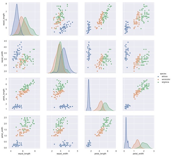
In the example below, from iris dataset we predict the species of flower based on the other measurements. In this case, the Species column would be considered as the feature.
在下面的示例中,我们从虹膜数据集中基于其他测量值来预测花朵的种类。 在这种情况下,“种类”列将被视为要素。
import seaborn as sns
iris = sns.load_dataset('iris')
%matplotlib inline
import seaborn as sns; sns.set()
sns.pairplot(iris, hue='species', height=3);
输出量 (Output)
X_iris = iris.drop('species', axis=1)
X_iris.shape
y_iris = iris['species']
y_iris.shape
输出量 (Output)
(150,4)
(150,)
Scikit Learn-估算器API (Scikit Learn - Estimator API)
In this chapter, we will learn about Estimator API (application programming interface). Let us begin by understanding what is an Estimator API.
在本章中,我们将学习Estimator API (应用程序编程接口)。 让我们首先了解什么是Estimator API。
什么是估算器API (What is Estimator API)
It is one of the main APIs implemented by Scikit-learn. It provides a consistent interface for a wide range of ML applications that’s why all machine learning algorithms in Scikit-Learn are implemented via Estimator API. The object that learns from the data (fitting the data) is an estimator. It can be used with any of the algorithms like classification, regression, clustering or even with a transformer, that extracts useful features from raw data.
它是Scikit-learn实现的主要API之一。 它为各种ML应用程序提供了一致的接口,这就是Scikit-Learn中所有机器学习算法都是通过Estimator API实现的原因。 从数据中学习(拟合数据)的对象是估计量。 它可以与分类,回归,聚类的任何算法一起使用,甚至可以与从原始数据中提取有用特征的转换器一起使用。
For fitting the data, all estimator objects expose a fit method that takes a dataset shown as follows −
为了拟合数据,所有估计器对象公开一个fit方法,该方法采用如下所示的数据集:
estimator.fit(data)
Next, all the parameters of an estimator can be set, as follows, when it is instantiated by the corresponding attribute.
接下来,当通过相应的属性实例化估算器时,可以如下设置估算器的所有参数。
estimator = Estimator (param1=1, param2=2)
estimator.param1
The output of the above would be 1.
上面的输出为1。
Once data is fitted with an estimator, parameters are estimated from the data at hand. Now, all the estimated parameters will be the attributes of the estimator object ending by an underscore as follows −
将数据与估算器拟合后,即可根据手头的数据估算参数。 现在,所有估计的参数将成为估计器对象的属性,以下划线结尾,如下所示:
estimator.estimated_param_
估算器API的使用 (Use of Estimator API)
Main uses of estimators are as follows −
估计器的主要用途如下-
模型的估计和解码 (Estimation and decoding of a model)
Estimator object is used for estimation and decoding of a model. Furthermore, the model is estimated as a deterministic function of the following −
估计器对象用于模型的估计和解码。 此外,该模型被估计为以下确定性函数-
The parameters which are provided in object construction.
对象构造中提供的参数。
The global random state (numpy.random) if the estimator’s random_state parameter is set to none.
如果估计器的random_state参数设置为none,则为全局随机状态(numpy.random)。
Any data passed to the most recent call to fit, fit_transform, or fit_predict.
传递给最新调用fit,fit_transform或fit_predict的任何数据。
Any data passed in a sequence of calls to partial_fit.
在对partial_fit的调用序列中传递的任何数据。
将非矩形数据表示映射到矩形数据 (Mapping non-rectangular data representation into rectangular data)
It maps a non-rectangular data representation into rectangular data. In simple words, it takes input where each sample is not represented as an array-like object of fixed length, and producing an array-like object of features for each sample.
它将非矩形数据表示形式映射为矩形数据。 简而言之,它接受输入,其中每个样本都不表示为固定长度的数组状对象,并为每个样本产生特征的数组状对象。
核心样本与外围样本之间的区别 (Distinction between core and outlying samples)
It models the distinction between core and outlying samples by using following methods −
它使用以下方法对核心样本和外围样本之间的区别进行建模-
fit
适合
fit_predict if transductive
fit_predict如果是转导的
predict if inductive
预测是否归纳
指导原则 (Guiding Principles)
While designing the Scikit-Learn API, following guiding principles kept in mind −
在设计Scikit-Learn API时,请牢记以下指导原则-
一致性 (Consistency)
This principle states that all the objects should share a common interface drawn from a limited set of methods. The documentation should also be consistent.
该原则指出,所有对象应该共享从一组有限的方法中提取的公共接口。 文档也应保持一致。
受限的对象层次 (Limited object hierarchy)
This guiding principle says −
这个指导原则说-
Algorithms should be represented by Python classes
算法应由Python类表示
Datasets should be represented in standard format like NumPy arrays, Pandas DataFrames, SciPy sparse matrix.
数据集应以标准格式表示,例如NumPy数组,Pandas DataFrames,SciPy稀疏矩阵。
Parameters names should use standard Python strings.
参数名称应使用标准的Python字符串。
组成 (Composition)
As we know that, ML algorithms can be expressed as the sequence of many fundamental algorithms. Scikit-learn makes use of these fundamental algorithms whenever needed.
众所周知,机器学习算法可以表示为许多基本算法的序列。 Scikit-learn会在需要时使用这些基本算法。
合理的默认值 (Sensible defaults)
According to this principle, the Scikit-learn library defines an appropriate default value whenever ML models require user-specified parameters.
根据此原理,只要ML模型需要用户指定的参数,Scikit-learn库就会定义适当的默认值。
检查 (Inspection)
As per this guiding principle, every specified parameter value is exposed as pubic attributes.
根据此指导原则,每个指定的参数值都公开为公共属性。
使用Estimator API的步骤 (Steps in using Estimator API)
Followings are the steps in using the Scikit-Learn estimator API −
以下是使用Scikit-Learn估计器API的步骤-
步骤1:选择模型类别 (Step 1: Choose a class of model)
In this first step, we need to choose a class of model. It can be done by importing the appropriate Estimator class from Scikit-learn.
在第一步中,我们需要选择一类模型。 可以通过从Scikit-learn导入适当的Estimator类来完成。
步骤2:选择模型超参数 (Step 2: Choose model hyperparameters)
In this step, we need to choose class model hyperparameters. It can be done by instantiating the class with desired values.
在这一步中,我们需要选择类模型超参数。 可以通过用所需的值实例化类来完成。
步骤3:整理资料 (Step 3: Arranging the data)
Next, we need to arrange the data into features matrix (X) and target vector(y).
接下来,我们需要将数据排列到特征矩阵(X)和目标向量(y)中。
步骤4:模型拟合 (Step 4: Model Fitting)
Now, we need to fit the model to your data. It can be done by calling fit() method of the model instance.
现在,我们需要使模型适合您的数据。 可以通过调用模型实例的fit()方法来完成。
步骤5:应用模型 (Step 5: Applying the model)
After fitting the model, we can apply it to new data. For supervised learning, use predict() method to predict the labels for unknown data. While for unsupervised learning, use predict() or transform() to infer properties of the data.
拟合模型后,我们可以将其应用于新数据。 对于监督学习,请使用predict()方法来预测未知数据的标签。 对于无监督学习,请使用predict()或transform()推断数据的属性。
监督学习的例子 (Supervised Learning Example)
Here, as an example of this process we are taking common case of fitting a line to (x,y) data i.e. simple linear regression.
在此,作为此过程的示例,我们以将线拟合到(x,y)数据的简单情况为例,即简单线性回归 。
First, we need to load the dataset, we are using iris dataset −
首先,我们需要加载数据集,我们使用虹膜数据集-
例 (Example)
import seaborn as sns
iris = sns.load_dataset('iris')
X_iris = iris.drop('species', axis = 1)
X_iris.shape
输出量 (Output)
(150, 4)
例 (Example)
y_iris = iris['species']
y_iris.shape
输出量 (Output)
(150,)
例 (Example)
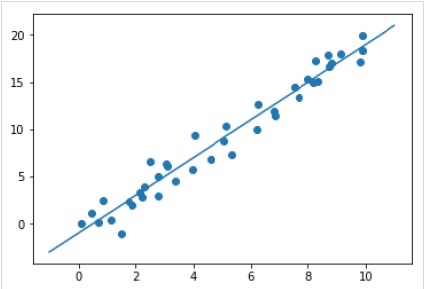
Now, for this regression example, we are going to use the following sample data −
现在,对于此回归示例,我们将使用以下样本数据-
%matplotlib inline
import matplotlib.pyplot as plt
import numpy as np
rng = np.random.RandomState(35)
x = 10*rng.rand(40)
y = 2*x-1+rng.randn(40)
plt.scatter(x,y);
输出量 (Output)

So, we have the above data for our linear regression example.
因此,对于线性回归示例,我们具有上述数据。
Now, with this data, we can apply the above-mentioned steps.
现在,利用这些数据,我们可以应用上述步骤。
选择一种型号 (Choose a class of model)
Here, to compute a simple linear regression model, we need to import the linear regression class as follows −
在这里,要计算一个简单的线性回归模型,我们需要导入线性回归类,如下所示:
from sklearn.linear_model import LinearRegression
选择模型超参数 (Choose model hyperparameters)
Once we choose a class of model, we need to make some important choices which are often represented as hyperparameters, or the parameters that must set before the model is fit to data. Here, for this example of linear regression, we would like to fit the intercept by using the fit_intercept hyperparameter as follows −
选择一类模型后,我们需要做出一些重要的选择,这些选择通常表示为超参数,或者是在模型适合数据之前必须设置的参数。 在这里,对于线性回归的示例,我们想通过使用fit_intercept超参数来拟合截距,如下所示:
Example
例
model = LinearRegression(fit_intercept = True)
model
Output
输出量
LinearRegression(copy_X = True, fit_intercept = True, n_jobs = None, normalize = False)
整理数据 (Arranging the data)
Now, as we know that our target variable y is in correct form i.e. a length n_samples array of 1-D. But, we need to reshape the feature matrix X to make it a matrix of size [n_samples, n_features]. It can be done as follows −
现在,我们知道我们的目标变量y的格式正确,即长度为1-D的n_samples数组。 但是,我们需要调整特征矩阵X的 形状,使其成为大小为[n_samples,n_features]的矩阵。 它可以做到如下-
Example
例
X = x[:, np.newaxis]
X.shape
Output
输出量
(40, 1)
模型拟合 (Model fitting)
Once, we arrange the data, it is time to fit the model i.e. to apply our model to data. This can be done with the help of fit() method as follows −
一旦我们整理了数据,就该对模型进行拟合了,即将模型应用于数据。 这可以借助fit()方法完成,如下所示:
Example
例
model.fit(X, y)
Output
输出量
LinearRegression(copy_X = True, fit_intercept = True, n_jobs = None,normalize = False)
In Scikit-learn, the fit() process have some trailing underscores.
在Scikit-learn中, fit()进程带有一些下划线。
For this example, the below parameter shows the slope of the simple linear fit of the data −
对于此示例,以下参数显示了数据的简单线性拟合的斜率-
Example
例
model.coef_
Output
输出量
array([1.99839352])
The below parameter represents the intercept of the simple linear fit to the data −
以下参数表示对数据的简单线性拟合的截距-
Example
例
model.intercept_
Output
输出量
-0.9895459457775022
将模型应用于新数据 (Applying the model to new data)
After training the model, we can apply it to new data. As the main task of supervised machine learning is to evaluate the model based on new data that is not the part of the training set. It can be done with the help of predict() method as follows −
训练模型后,我们可以将其应用于新数据。 监督式机器学习的主要任务是根据不是训练集一部分的新数据评估模型。 可以借助预测()方法完成以下操作-
Example
例
xfit = np.linspace(-1, 11)
Xfit = xfit[:, np.newaxis]
yfit = model.predict(Xfit)
plt.scatter(x, y)
plt.plot(xfit, yfit);
Output
输出量
完整的工作/可执行示例 (Complete working/executable example)
%matplotlib inline
import matplotlib.pyplot as plt
import numpy as np
import seaborn as sns

iris = sns.load_dataset('iris')
X_iris = iris.drop('species', axis = 1)
X_iris.shape
y_iris = iris['species']
y_iris.shape

rng = np.random.RandomState(35)
x = 10*rng.rand(40)
y = 2*x-1+rng.randn(40)
plt.scatter(x,y);
from sklearn.linear_model import LinearRegression
model = LinearRegression(fit_intercept=True)
model
X = x[:, np.newaxis]
X.shape

model.fit(X, y)
model.coef_
model.intercept_

xfit = np.linspace(-1, 11)
Xfit = xfit[:, np.newaxis]
yfit = model.predict(Xfit)
plt.scatter(x, y)
plt.plot(xfit, yfit);
无监督学习示例 (Unsupervised Learning Example)
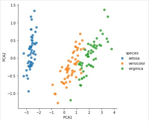
Here, as an example of this process we are taking common case of reducing the dimensionality of the Iris dataset so that we can visualize it more easily. For this example, we are going to use principal component analysis (PCA), a fast-linear dimensionality reduction technique.
在此,作为此过程的示例,我们以降低Iris数据集的维数为例,以便我们可以更轻松地对其进行可视化。 对于此示例,我们将使用主成分分析(PCA),一种快速线性降维技术。
Like the above given example, we can load and plot the random data from iris dataset. After that we can follow the steps as below −
像上面给出的示例一样,我们可以从虹膜数据集中加载并绘制随机数据。 之后,我们可以按照以下步骤操作-
选择一种型号 (Choose a class of model)
from sklearn.decomposition import PCA
选择模型超参数 (Choose model hyperparameters)
Example
例
model = PCA(n_components=2)
model
Output
输出量
PCA(copy = True, iterated_power = 'auto', n_components = 2, random_state = None,
   svd_solver = 'auto', tol = 0.0, whiten = False)
模型拟合 (Model fitting)
Example
例
model.fit(X_iris)
Output
输出量
PCA(copy = True, iterated_power = 'auto', n_components = 2, random_state = None,
   svd_solver = 'auto', tol = 0.0, whiten = False)
将数据转换为二维 (Transform the data to two-dimensional)
Example
例
X_2D = model.transform(X_iris)
Now, we can plot the result as follows −
现在,我们可以将结果绘制如下:
Output
输出量
iris['PCA1'] = X_2D[:, 0]
iris['PCA2'] = X_2D[:, 1]
sns.lmplot("PCA1", "PCA2", hue = 'species', data = iris, fit_reg = False);
Output
输出量
完整的工作/可执行示例 (Complete working/executable example)
%matplotlib inline
import matplotlib.pyplot as plt
import numpy as np
import seaborn as sns

iris = sns.load_dataset('iris')
X_iris = iris.drop('species', axis = 1)
X_iris.shape
y_iris = iris['species']
y_iris.shape
rng = np.random.RandomState(35)
x = 10*rng.rand(40)
y = 2*x-1+rng.randn(40)
plt.scatter(x,y);
from sklearn.decomposition import PCA

model = PCA(n_components=2)
model
model.fit(X_iris)
X_2D = model.transform(X_iris)
iris['PCA1'] = X_2D[:, 0]
iris['PCA2'] = X_2D[:, 1]
sns.lmplot("PCA1", "PCA2", hue='species', data=iris, fit_reg=False);
Scikit Learn-约定 (Scikit Learn - Conventions)
Scikit-learn’s objects share a uniform basic API that consists of the following three complementary interfaces −
Scikit-learn的对象共享一个统一的基本API,该API由以下三个互补接口组成-
Estimator interface − It is for building and fitting the models.
估计器接口 -用于构建和拟合模型。
Predictor interface − It is for making predictions.
预测器接口 -用于进行预测。
Transformer interface − It is for converting data.
变压器接口 -用于转换数据。
The APIs adopt simple conventions and the design choices have been guided in a manner to avoid the proliferation of framework code.
这些API采用简单的约定,并且以避免框架代码泛滥的方式指导了设计选择。
公约目的 (Purpose of Conventions)
The purpose of conventions is to make sure that the API stick to the following broad principles −
约定的目的是确保API遵循以下广泛原则-
Consistency − All the objects whether they are basic, or composite must share a consistent interface which further composed of a limited set of methods.
一致性 -所有对象(无论是基础对象还是复合对象)都必须共享一致的接口,该接口进一步由一组有限的方法组成。
Inspection − Constructor parameters and parameters values determined by learning algorithm should be stored and exposed as public attributes.
检查 -构造函数参数和由学习算法确定的参数值应存储并公开为公共属性。
Non-proliferation of classes − Datasets should be represented as NumPy arrays or Scipy sparse matrix whereas hyper-parameters names and values should be represented as standard Python strings to avoid the proliferation of framework code.
类的不扩散 -数据集应表示为NumPy数组或Scipy稀疏矩阵,而超参数名称和值应表示为标准Python字符串,以避免框架代码的泛滥。
Composition − The algorithms whether they are expressible as sequences or combinations of transformations to the data or naturally viewed as meta-algorithms parameterized on other algorithms, should be implemented and composed from existing building blocks.
组合 -无论是将算法表达为数据转换的序列还是转换的组合,或者自然地视为在其他算法上参数化的元算法,都应从现有的构建模块中实施并组成。
Sensible defaults − In scikit-learn whenever an operation requires a user-defined parameter, an appropriate default value is defined. This default value should cause the operation to be performed in a sensible way, for example, giving a base-line solution for the task at hand.
合理的默认值 -在scikit-learn中,每当操作需要用户定义的参数时,就会定义适当的默认值。 此默认值应使操作以明智的方式执行,例如,为手头的任务提供基线解决方案。
各种约定 (Various Conventions)
The conventions available in Sklearn are explained below −
Sklearn中可用的约定在下面进行了解释-
型铸 (Type casting)
It states that the input should be cast to float64. In the following example, in which sklearn.random_projection module used to reduce the dimensionality of the data, will explain it −
它指出输入应强制转换为float64 。 在以下示例中,其中sklearn.random_projection模块用于降低数据的维数,将对此进行解释-
Example
例
import numpy as np
from sklearn import random_projection
rannge = np.random.RandomState(0)
X = range.rand(10,2000)
X = np.array(X, dtype = 'float32')
X.dtype
Transformer_data = random_projection.GaussianRandomProjection()
X_new = transformer.fit_transform(X)
X_new.dtype
Output
输出量
dtype('float32')
dtype('float64')
In the above example, we can see that X is float32 which is cast to float64 by fit_transform(X).
在上面的示例中,我们可以看到X是float32 ,它由fit_transform(X)强制转换为float64 。
改装和更新参数 (Refitting & Updating Parameters)
Hyper-parameters of an estimator can be updated and refitted after it has been constructed via the set_params() method. Let’s see the following example to understand it −
通过set_params()方法构造估算器的超参数后,可以对其进行更新和调整。 让我们看下面的例子来理解它-
Example
例
import numpy as np
from sklearn.datasets import load_iris
from sklearn.svm import SVC
X, y = load_iris(return_X_y = True)
clf = SVC()
clf.set_params(kernel = 'linear').fit(X, y)
clf.predict(X[:5])
Output
输出量
array([0, 0, 0, 0, 0])
Once the estimator has been constructed, above code will change the default kernel rbf to linear via SVC.set_params().
一旦估计已经构造,上面的代码将更改默认内核RBF到线性经由SVC.set_params()。
Now, the following code will change back the kernel to rbf to refit the estimator and to make a second prediction.
现在,以下代码将把内核改回rbf,以重新拟合估计器并进行第二次预测。
Example
例
clf.set_params(kernel = 'rbf', gamma = 'scale').fit(X, y)
clf.predict(X[:5])
Output
输出量
array([0, 0, 0, 0, 0])
完整的代码 (Complete code)
The following is the complete executable program −
以下是完整的可执行程序-
import numpy as np
from sklearn.datasets import load_iris
from sklearn.svm import SVC
X, y = load_iris(return_X_y = True)
clf = SVC()
clf.set_params(kernel = 'linear').fit(X, y)
clf.predict(X[:5])
clf.set_params(kernel = 'rbf', gamma = 'scale').fit(X, y)
clf.predict(X[:5])
多类别和多标签拟合 (Multiclass & Multilabel fitting)
In case of multiclass fitting, both learning and the prediction tasks are dependent on the format of the target data fit upon. The module used is sklearn.multiclass. Check the example below, where multiclass classifier is fit on a 1d array.
在进行多类拟合的情况下,学习任务和预测任务都取决于适合的目标数据的格式。 使用的模块是sklearn.multiclass 。 检查下面的示例,其中多类分类器适合一维数组。
Example
例
from sklearn.svm import SVC
from sklearn.multiclass import OneVsRestClassifier
from sklearn.preprocessing import LabelBinarizer
X = [[1, 2], [3, 4], [4, 5], [5, 2], [1, 1]]
y = [0, 0, 1, 1, 2]
classif = OneVsRestClassifier(estimator = SVC(gamma = 'scale',random_state = 0))
classif.fit(X, y).predict(X)
Output
输出量
array([0, 0, 1, 1, 2])
In the above example, classifier is fit on one dimensional array of multiclass labels and the predict() method hence provides corresponding multiclass prediction. But on the other hand, it is also possible to fit upon a two-dimensional array of binary label indicators as follows −
在上面的示例中,分类器适合多类标签的一维数组,并且predict()方法因此提供了相应的多类预测。 但另一方面,也可以将二进制标签指示符的二维数组拟合如下:
Example
例
 最低0.47元/天 解锁文章


 7778
7778


 被折叠的 条评论
为什么被折叠?
被折叠的 条评论
为什么被折叠?
 到【灌水乐园】发言


