


去年,我遇到了Twitter的异常检测库 ,但还没有理由进行测试运行,因此,将我的博客帖子频率数据整理成形状后,我认为通过算法运行它会很有趣。
我想看看它是否可以检测到一段时间内发帖数量明显不同的情况–根据结果,我真的没有采取任何行动,这比任何其他事情都更具好奇心!
首先,我们需要安装该库。 它不在CRAN上,因此我们需要使用devtools从github仓库中安装它:
install.packages("devtools")
devtools::install_github("twitter/AnomalyDetection")
library(AnomalyDetection)
预期的数据格式为两列,一列包含时间戳,另一列包含计数。 例如,使用添加库时作用域内的“ raw_data”数据框:
> library(dplyr)
> raw_data %>% head()
            timestamp   count
1 1980-09-25 14:01:00 182.478
2 1980-09-25 14:02:00 176.231
3 1980-09-25 14:03:00 183.917
4 1980-09-25 14:04:00 177.798
5 1980-09-25 14:05:00 165.469
6 1980-09-25 14:06:00 181.878
在我们的示例中,时间戳记将是一周的开始日期,并计算该周中的帖子数。 但是首先让我们练习一下使用固定数据调用异常函数:
res = AnomalyDetectionTs(raw_data, max_anoms=0.02, direction='both', plot=TRUE)
res$plot 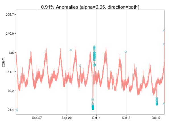
通过这种可视化,我们了解到应该期望识别出较高和较低的异常值。 让我们尝试一下博客文章的发布数据。
我们需要使数据成形,因此我们首先要按(周,年)对来获取博客文章的数量:
> df %>% sample_n(5)
                                                           title                date
1425                            Coding: Copy/Paste then refactor 2009-10-31 07:54:31
783  Neo4j 2.0.0-M06 -> 2.0.0-RC1: Working with path expressions 2013-11-23 10:30:41
960                                        R: Removing for loops 2015-04-18 23:53:20
966   R: dplyr - Error in (list: invalid subscript type 'double' 2015-04-27 22:34:43
343                     Parsing XML from the unix terminal/shell 2011-09-03 23:42:11

> byWeek = df %>%
    mutate(year = year(date), week = week(date)) %>%
    group_by(week, year) %>% summarise(n = n()) %>%
    ungroup() %>% arrange(desc(n))

> byWeek %>% sample_n(5)
Source: local data frame [5 x 3]

  week year n
1   44 2009 6
2   37 2011 4
3   39 2012 3
4    7 2013 4
5    6 2010 6
大。 下一步是将该数据框转换为包含日期的数据框,该日期代表该周的开始日期和帖子数:
> data = byWeek %>%
    mutate(start_of_week = calculate_start_of_week(week, year)) %>%
    filter(start_of_week > ymd("2008-07-01")) %>%
    select(start_of_week, n)

> data %>% sample_n(5)
Source: local data frame [5 x 2]

  start_of_week n
1    2010-09-10 4
2    2013-04-09 4
3    2010-04-30 6
4    2012-03-11 3
5    2014-12-03 3
现在我们准备将其插入异常检测功能:
res = AnomalyDetectionTs(data,
                         max_anoms=0.02,
                         direction='both',
                         plot=TRUE)
res$plot 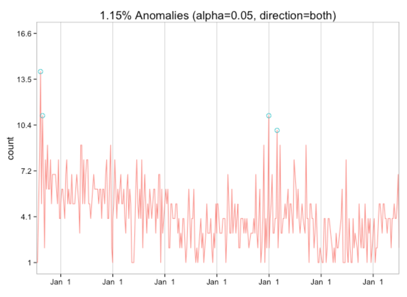
有趣的是,我似乎没有任何低端异常现象–当我刚开始写作时,有几个非常高频率的星期,而我认为其他几个星期中有一个我特别无聊的除夕夜!
如果我们按月分组,那么只有第一个月是一个异常值:
data = byMonth %>%
  mutate(start_of_month = ymd(paste(year, month, 1, sep="-"))) %>%
  filter(start_of_month > ymd("2008-07-01")) %>%
  select(start_of_month, n)
res = AnomalyDetectionTs(data,
                         max_anoms=0.02,
                         direction='both',
                         #longterm = TRUE,
                         plot=TRUE)
res$plot 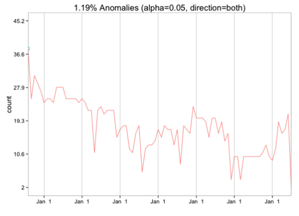
我不确定就异常检测而言还可以做些什么,但是如果您有任何想法,请告诉我!
翻译自: https://www.javacodegeeks.com/2015/07/r-blog-post-frequency-anomaly-detection.html


 736
736

 被折叠的 条评论
为什么被折叠?
被折叠的 条评论
为什么被折叠?
 到【灌水乐园】发言


