


logistic回归预测
在此博客文章中,我将帮助您开始使用Apache Spark的spark.ml Logistic回归来预测癌症恶性程度。
Spark的spark.ml库目标是在DataFrames之上提供一组API,以帮助用户创建和调整机器学习工作流程或管道。 将spark.ml与DataFrames一起使用可通过智能优化提高性能。
分类
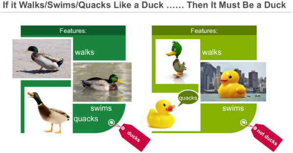
分类是一类有监督的机器学习算法,该算法基于已知项目的标记示例(例如,已知为恶性的观察结果)来识别该项目属于哪个类别(例如,癌组织观察结果是否为恶性)。 )。 分类采用具有已知标签和预定功能的一组数据,并学习如何基于该信息对新记录进行标签。 功能就是您提出的“如果有问题”。 标签是这些问题的答案。 在下面的示例中,如果它像鸭子一样走路,游泳和嘎嘎叫声,则标签为“鸭子”。
让我们来看一个癌组织观察的例子:
- 我们要预测什么?
- 样本观察结果是否为恶性。
- 您可以用来预测的“如果有问题”或属性是什么?
- 组织样本特征:团块厚度,细胞大小均匀性,细胞形状均匀性,边缘附着力,单个上皮细胞大小,裸核,温和染色质,正常核仁,线粒体。
逻辑回归
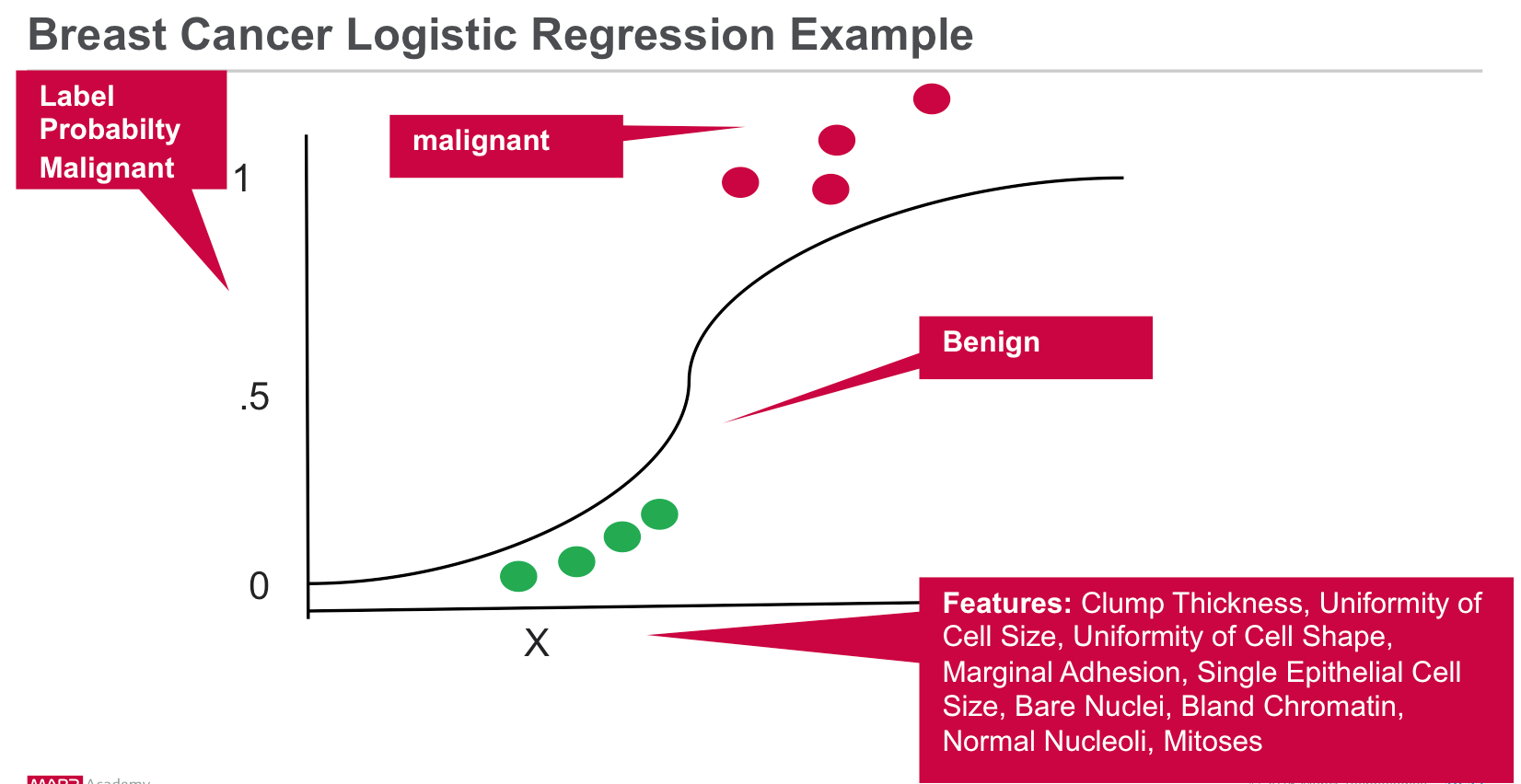
Logistic回归是一种流行的预测二进制响应的方法。 这是广义线性模型的一种特殊情况,可以预测结果的可能性。 Logistic回归通过使用Logistic函数估计概率来度量Y“标签”和X“特征”之间的关系。 该模型预测用于预测标签类别的概率。
使用Spark机器学习场景分析癌症观察结果
我们的数据来自威斯康星州诊断性乳腺癌(WDBC)数据集,该数据集根据9种特征将乳腺肿瘤病例分类为良性或恶性,以预测诊断。 对于每个癌症观察,我们都有以下信息:
1. Sample code number: id number
2. Clump Thickness: 1 - 10
3. Uniformity of Cell Size: 1 - 10
4. Uniformity of Cell Shape: 1 - 10
5. Marginal Adhesion: 1 - 10
6. Single Epithelial Cell Size: 1 - 10
7. Bare Nuclei: 1 - 10
8. Bland Chromatin: 1 - 10
9. Normal Nucleoli: 1 - 10
10. Mitoses: 1 - 10
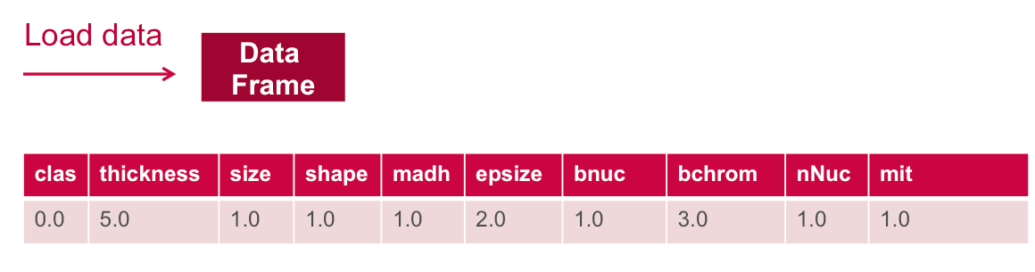
11. Class: (2 for benign, 4 for malignant)癌症观察csv文件具有以下格式:
1000025,5,1,1,1,2,1,3,1,1,2
1002945,5,4,4,5,7,10,3,2,1,2
1015425,3,1,1,1,2,2,3,1,1,2
在这种情况下,我们将基于以下特征构建一个逻辑回归模型来预测恶性肿瘤的标签/分类:
- 标签→恶性或良性(1或0)
- 特征→{丛集厚度,细胞大小均匀性,细胞形状均匀性,边缘粘附性,单上皮细胞大小,裸核,温和染色质,正常核仁,线粒体}
Spark ML提供了一组基于DataFrames的统一高级API。 Spark ML的主要概念是:
- DataFrame:ML API使用Spark SQL中的DataFrames作为ML数据集。
- 变压器:变压器是一种将一个DataFrame转换为另一个DataFrame的算法。 例如,将具有特征的DataFrame转换为具有预测的DataFrame。
- 估计器:估计器是一种算法,可以适合于DataFrame来生成Transformer。 例如,在DataFrame上进行训练/调整并生成模型。
- 管道:管道将多个Transformer和Estimators链接在一起,以指定ML工作流程。
- ParamMaps:要选择的参数,有时也称为“参数网格”。
- 评估者:衡量拟合模型对保留的测试数据的表现的度量。
- CrossValidator:确定最佳的ParamMap,并使用最佳的ParamMap和整个数据集重新拟合Estimator。
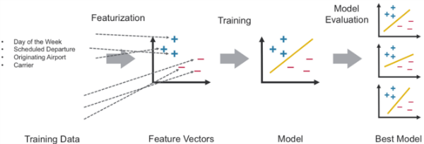
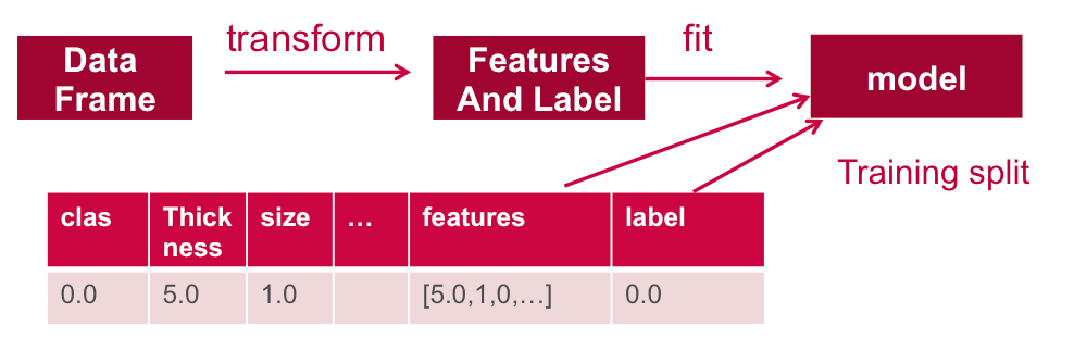
在此示例中,将使用如下所示的Spark ML工作流: 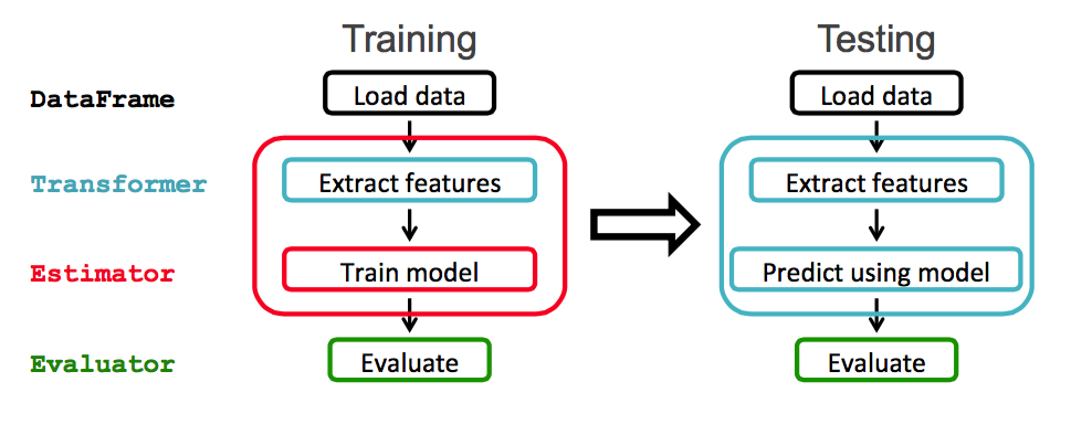
软件
本教程将在Spark 1.6.1上运行
- 您可以从此处下载代码和数据以运行这些示例: https : //github.com/caroljmcdonald/spark-ml-lr-cancer
- 使用spark-shell命令启动后,本文中的示例可以在Spark shell中运行。
- 您还可以按照独立的应用程序运行代码,如MapR Sandbox上的Spark入门教程中所述。
如使用Mapr Sandbox上的Spark入门所述 ,使用密码为userid user01的用户登录到MapR Sandbox。 使用scp将样本数据文件复制到沙箱主目录/ user / user01。 (请注意,您可能必须在沙箱上更新Spark版本),使用以下命令启动Spark Shell:
$spark-shell --master local[1]从csv文件加载和解析数据
首先,我们将导入机器学习包。
(在代码框中,注释为绿色,输出为蓝色)
import org.apache.spark._
import org.apache.spark.rdd.RDD
import org.apache.spark.sql.SQLContext
import org.apache.spark.ml.feature.StringIndexer
import org.apache.spark.ml.feature.VectorAssembler
import org.apache.spark.ml.classification.BinaryLogisticRegressionSummary
import org.apache.spark.ml.evaluation.BinaryClassificationEvaluator
import org.apache.spark.ml.classification.LogisticRegression
import org.apache.spark.ml.feature.StringIndexer
import org.apache.spark.ml.feature.VectorAssembler
import sqlContext.implicits._
import sqlContext._
import org.apache.spark.sql.functions._
import org.apache.spark.mllib.linalg.DenseVector
import org.apache.spark.mllib.evaluation.BinaryClassificationMetrics
我们使用Scala案例类来定义与csv数据文件中的一行相对应的架构。
// define the Cancer Observation Schema
case class Obs(clas: Double, thickness: Double, size: Double, shape: Double, madh: Double, epsize: Double, bnuc: Double, bchrom: Double, nNuc: Double, mit: Double)
下面的函数将数据文件中的一行解析为癌症观察类。
// function to create a Obs class from an Array of Double.Class Malignant 4 is changed to 1
def parseObs(line: Array[Double]): Obs = {
    Obs(
      if (line(9) == 4.0) 1 else 0, line(0), line(1), line(2), line(3), line(4), line(5), line(6), line(7), line(8)
    )
}
// function to transform an RDD of Strings into an RDD of Double, filter lines with ?, remove first column
def parseRDD(rdd: RDD[String]): RDD[Array[Double]] = {
    rdd.map(_.split(",")).filter(_(6) != "?").map(_.drop(1)).map(_.map(_.toDouble))
}
下面,我们将csv文件中的数据加载到字符串的RDD中。 然后,我们在rdd上使用map转换,它将应用ParseRDD函数将RDD中的每个String元素转换为Double数组。 然后,我们使用另一个映射变换,该变换将应用ParseObs函数将RDD中的每个Double数组变换为一个癌观测对象数组。 toDF()方法将数组[[癌症观察]]的RDD转换为具有癌症观察类模式的数据框。
// load the data into a DataFrame
val rdd = sc.textFile("data/breast_cancer_wisconsin_data.txt")
val obsRDD = parseRDD(rdd).map(parseObs)
val obsDF = obsRDD.toDF().cache()
obsDF.registerTempTable("obs")
DataFrame printSchema()以树格式将模式打印到控制台
// Return the schema of this DataFrame
obsDF.printSchema

root
 |-- clas: double (nullable = false)
 |-- thickness: double (nullable = false)
 |-- size: double (nullable = false)
 |-- shape: double (nullable = false)
 |-- madh: double (nullable = false)
 |-- epsize: double (nullable = false)
 |-- bnuc: double (nullable = false)
 |-- bchrom: double (nullable = false)
 |-- nNuc: double (nullable = false)
 |-- mit: double (nullable = false)

// Display the top 20 rows of DataFrame
obsDF.show


+----+---------+----+-----+----+------+----+------+----+---+
|clas|thickness|size|shape|madh|epsize|bnuc|bchrom|nNuc|mit|
+----+---------+----+-----+----+------+----+------+----+---+
| 0.0|      5.0| 1.0|  1.0| 1.0|   2.0| 1.0|   3.0| 1.0|1.0|
| 0.0|      5.0| 4.0|  4.0| 5.0|   7.0|10.0|   3.0| 2.0|1.0|
| 0.0|      3.0| 1.0|  1.0| 1.0|   2.0| 2.0|   3.0| 1.0|1.0|
...
+----+---------+----+-----+----+------+----+------+----+---+
only showing top 20 rows
实例化DataFrame之后,可以使用SQL查询对其进行查询。 以下是一些使用Scala DataFrame API的示例查询:
描述计算厚度列的统计信息,包括计数,平均值,stddev,最小值和最大值
//  computes statistics for thickness
obsDF.describe("thickness").show

+-------+------------------+
|summary|         thickness|
+-------+------------------+
|  count|               683|
|   mean|  4.44216691068814|
| stddev|2.8207613188371288|
|    min|               1.0|
|    max|              10.0|
+-------+------------------+


// compute the avg thickness, size, shape grouped by clas (malignant or not)
sqlContext.sql("SELECT clas, avg(thickness) as avgthickness, avg(size) as avgsize, avg(shape) as avgshape FROM obs GROUP BY clas ").show

+----+-----------------+------------------+------------------+
|clas|     avgthickness|           avgsize|          avgshape|
+----+-----------------+------------------+------------------+
| 1.0|7.188284518828452| 6.577405857740586| 6.560669456066946|
| 0.0|2.963963963963964|1.3063063063063063|1.4144144144144144|
+----+-----------------+------------------+------------------+

// compute avg thickness grouped by clas (malignant or not)
obsDF.groupBy("clas").avg("thickness").show

+----+-----------------+
|clas|   avg(thickness)|
+----+-----------------+
| 1.0|7.188284518828452|
| 0.0|2.963963963963964|
+----+-----------------+
提取功能
要构建分类器模型,您首先要提取最有助于分类的特征。 在癌症数据集中,数据被标记为两个类别-1(恶性)和0(非恶性)。
每个项目的功能均包含以下字段:
- 标签→恶性:0或1
- 功能→{“厚度”,“大小”,“形状”,“ madh”,“ epsize”,“ bnuc”,“ bchrom”,“ nNuc”,“ mit”}
定义要素数组
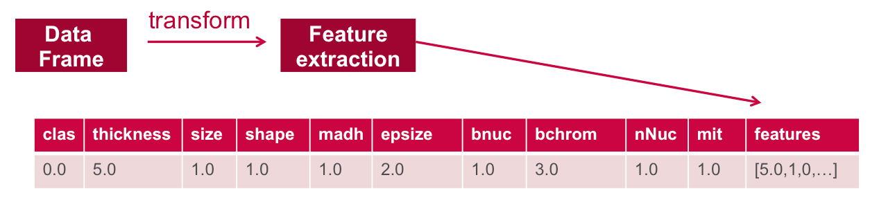
为了让机器学习算法使用特征,对特征进行转换并将其放入特征向量中,特征向量是代表每个特征值的数字向量。
在VectorAssembler下方,用于转换和返回一个新的DataFrame,该向量框架具有vector列中的所有功能列
//define the feature columns to put in the feature vector
val featureCols = Array("thickness", "size", "shape", "madh", "epsize", "bnuc", "bchrom", "nNuc", "mit")
//set the input and output column names
val assembler = new VectorAssembler().setInputCols(featureCols).setOutputCol("features")
//return a dataframe with all of the feature columns in a vector column
val df2 = assembler.transform(obsDF)
// the transform method produced a new column: features.
df2.show
+----+---------+----+-----+----+------+----+------+----+---+--------------------+
|clas|thickness|size|shape|madh|epsize|bnuc|bchrom|nNuc|mit| features|
+----+---------+----+-----+----+------+----+------+----+---+--------------------+
| 0.0| 5.0| 1.0| 1.0| 1.0| 2.0| 1.0| 3.0| 1.0|1.0|[5.0,1.0,1.0,1.0,...|
| 0.0| 5.0| 4.0| 4.0| 5.0| 7.0|10.0| 3.0| 2.0|1.0|[5.0,4.0,4.0,5.0,...|
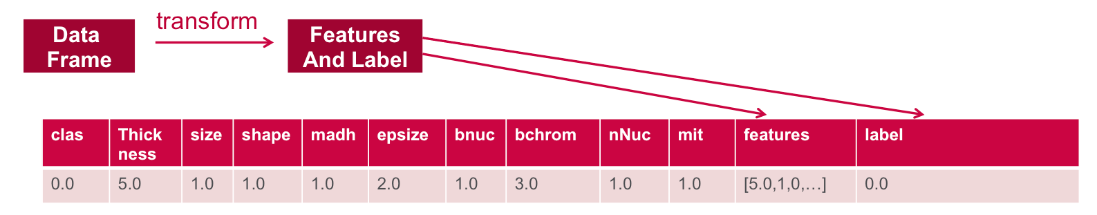
| 1.0| 8.0|10.0| 10.0| 8.0| 7.0|10.0| 9.0| 7.0|1.0|[8.0,10.0,10.0,8....|接下来,我们使用StringIndexer返回添加了clas(是否为恶性)列作为label的Dataframe。
// Create a label column with the StringIndexer
val labelIndexer = new StringIndexer().setInputCol("clas").setOutputCol("label")
val df3 = labelIndexer.fit(df2).transform(df2)
// the transform method produced a new column: label.
df3.show
+----+---------+----+-----+----+------+----+------+----+---+--------------------+-----+
|clas|thickness|size|shape|madh|epsize|bnuc|bchrom|nNuc|mit| features|label|
+----+---------+----+-----+----+------+----+------+----+---+--------------------+-----+
| 0.0| 5.0| 1.0| 1.0| 1.0| 2.0| 1.0| 3.0| 1.0|1.0|[5.0,1.0,1.0,1.0,...| 0.0|
| 0.0| 5.0| 4.0| 4.0| 5.0| 7.0|10.0| 3.0| 2.0|1.0|[5.0,4.0,4.0,5.0,...| 0.0|
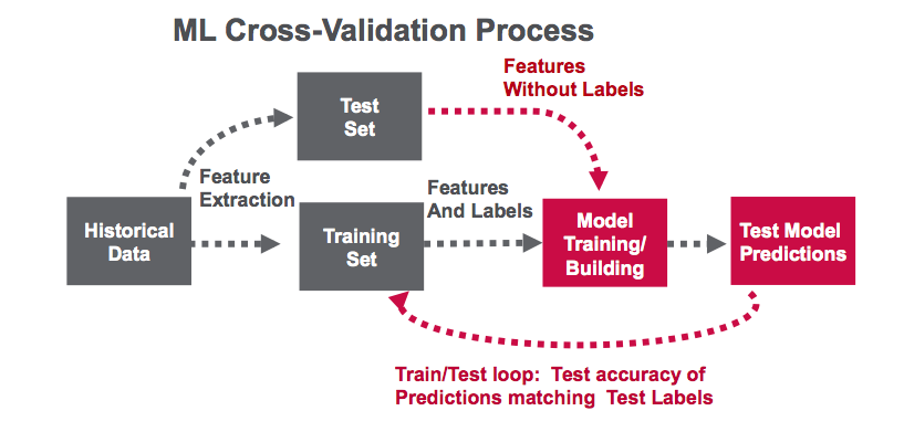
| 0.0| 3.0| 1.0| 1.0| 1.0| 2.0| 2.0| 3.0| 1.0|1.0|[3.0,1.0,1.0,1.0,...| 0.0|下面的数据。 它分为训练数据集和测试数据集。 70%的数据用于训练模型,而30%的数据用于测试。
//  split the dataframe into training and test data
val splitSeed = 5043
val Array(trainingData, testData) = df3.randomSplit(Array(0.7, 0.3), splitSeed)
训练模型
接下来,我们使用弹性网正则化训练逻辑回归模型
通过在输入要素和与那些要素相关的标记输出之间建立关联来训练模型。
// create the classifier,  set parameters for training
val lr = new LogisticRegression().setMaxIter(10).setRegParam(0.3).setElasticNetParam(0.8)
//  use logistic regression to train (fit) the model with the training data
val model = lr.fit(trainingData)

// Print the coefficients and intercept for logistic regression
println(s"Coefficients: ${model.coefficients} Intercept: ${model.intercept}")


Coefficients: (9,[1,2,5,6],[0.06503554553146387,0.07181362361391264,0.07583963853124673,0.0012675057388232965]) Intercept: -1.39319142312609
测试模型
接下来,我们使用测试数据来获得预测。
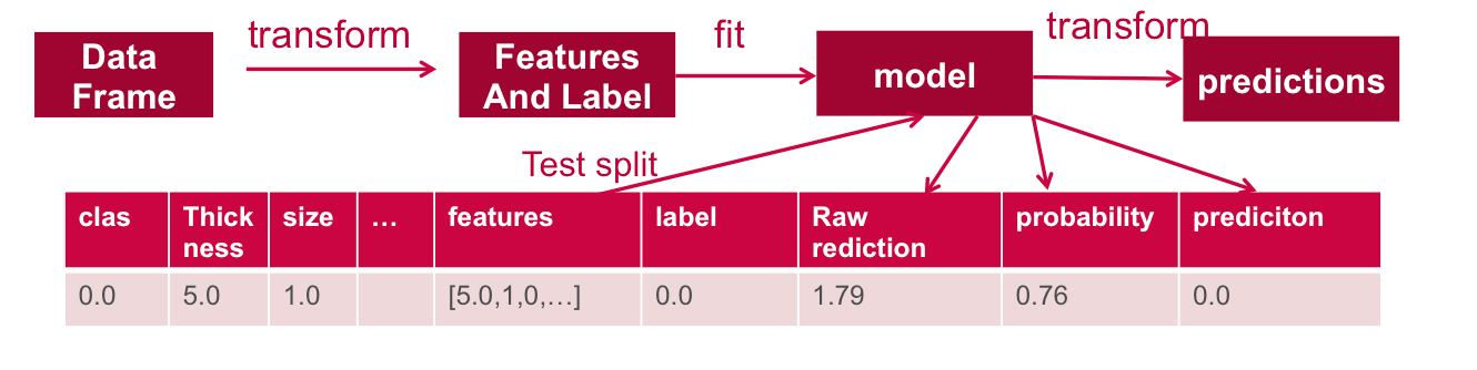
// run the  model on test features to get predictions
val predictions = model.transform(testData)
//As you can see, the previous model transform produced a new columns: rawPrediction, probablity and prediction.
predictions.show

+----+---------+----+-----+----+------+----+------+----+---+--------------------+-----+--------------------+--------------------+----------+
|clas|thickness|size|shape|madh|epsize|bnuc|bchrom|nNuc|mit|            features|label|       rawPrediction|         probability|prediction|
+----+---------+----+-----+----+------+----+------+----+---+--------------------+-----+--------------------+--------------------+----------+
| 0.0|      1.0| 1.0|  1.0| 1.0|   1.0| 1.0|   1.0| 3.0|1.0|[1.0,1.0,1.0,1.0,...|  0.0|[1.17923510971064...|[0.76481024658406...|       0.0|
| 0.0|      1.0| 1.0|  1.0| 1.0|   1.0| 1.0|   3.0| 1.0|1.0|[1.0,1.0,1.0,1.0,...|  0.0|[1.17670009823299...|[0.76435395397908...|       0.0|
| 0.0|      1.0| 1.0|  1.0| 1.0|   1.0| 1.0|   3.0| 1.0|1.0|[1.0,1.0,1.0,1.0,...|  0.0|[1.17670009823299...|[0.76435395397908...|       0.0|
| 0.0|      1.0| 1.0|  1.0| 1.0|   2.0| 1.0|   1.0| 1.0|1.0|[1.0,1.0,1.0,1.0,...|  0.0|[1.17923510971064...|[0.76481024658406...|       0.0|
| 0.0|      1.0| 1.0|  1.0| 1.0|   2.0| 1.0|   2.0| 1.0|1.0|[1.0,1.0,1.0,1.0,...|  0.0|[1.17796760397182...|[0.76458217679258...|       0.0|
+----+---------+----+-----+----+------+----+------+----+---+--------------------+-----+--------------------+--------------------+----------+
下面我们评估预测,我们使用BinaryClassificationEvaluator通过比较测试标签列和测试预测列来返回精度指标。 在这种情况下,评估返回99%的精度。
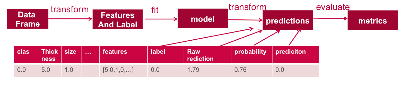
//A common metric used for logistic regression is area under the ROC curve (AUC). We can use the BinaryClasssificationEvaluator to obtain the AUC
// create an Evaluator for binary classification, which expects two input columns: rawPrediction and label.
val evaluator = new BinaryClassificationEvaluator().setLabelCol("label").setRawPredictionCol("rawPrediction").setMetricName("areaUnderROC")
// Evaluates predictions and returns a scalar metric areaUnderROC(larger is better).
val accuracy = evaluator.evaluate(predictions)
accuracy: Double = 0.9926910299003322
下面我们计算更多指标。 错误和真实的正面和负面预测的数量也很有用:
- 真阳性是模型正确预测肿瘤为恶性的频率
- 假阳性是模型多久预测一次肿瘤是良性的恶性肿瘤
- 真阴性表明模型如何正确预测肿瘤是良性的
- 假阴性表明模型多久预测一次肿瘤实际上是恶性的
// Calculate Metrics
val lp = predictions.select( "label", "prediction")
val counttotal = predictions.count()
val correct = lp.filter($"label" === $"prediction").count()
val wrong = lp.filter(not($"label" === $"prediction")).count()
val truep = lp.filter($"prediction" === 0.0).filter($"label" === $"prediction").count()
val falseN = lp.filter($"prediction" === 0.0).filter(not($"label" === $"prediction")).count()
val falseP = lp.filter($"prediction" === 1.0).filter(not($"label" === $"prediction")).count()
val ratioWrong=wrong.toDouble/counttotal.toDouble
val ratioCorrect=correct.toDouble/counttotal.toDouble


counttotal: Long = 199
correct: Long = 168
wrong: Long = 31
truep: Long = 128
falseN: Long = 30
falseP: Long = 1
ratioWrong: Double = 0.15577889447236182
ratioCorrect: Double = 0.8442211055276382


// use MLlib to evaluate, convert DF to RDD
val  predictionAndLabels =predictions.select("rawPrediction", "label").rdd.map(x => (x(0).asInstanceOf[DenseVector](1), x(1).asInstanceOf[Double]))
val metrics = new BinaryClassificationMetrics(predictionAndLabels)
println("area under the precision-recall curve: " + metrics.areaUnderPR)
println("area under the receiver operating characteristic (ROC) curve : " + metrics.areaUnderROC)
// A Precision-Recall curve plots (precision, recall) points for different threshold values, while a receiver operating characteristic, or ROC, curve plots (recall, false positive rate) points. The closer  the area Under ROC is to 1, the better the model is making predictions.

area under the precision-recall curve: 0.9828385182615946
area under the receiver operating characteristic (ROC) curve : 0.9926910299003322
想了解更多?
在此博客文章中,我们向您展示了如何开始使用Apache Spark的机器学习Logistic回归进行分类。 如果您对本教程还有其他疑问,请在下面的评论部分中提问。
logistic回归预测


 749
749


 被折叠的 条评论
为什么被折叠?
被折叠的 条评论
为什么被折叠?
 到【灌水乐园】发言


