Coursera深度学习：Planar data classification with one hidden layer

一、load the data

        在给定数据集中，包含X和Y两个numpy array，其中X储存features(x1, x2)，Y储存labels (red:0, blue:1)。

X, Y = load_planar_dataset()

shape_X = X.shape # (2,400)
shape_Y = Y.shape  # (1,400)
m = shape_X[1]    # m=400

        利用如下代码将数据集进行可视化

# Visualize the data:
plt.scatter(X[0, :], X[1, :], c=Y, s=40, cmap=plt.cm.Spectral);

        

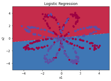
二、Simple Logistic Regression

        如果简单的使用logistic regression，我们得到的结果如下：（此处不再对logistic regression 的模型进行说明，详细可见--Logistic Regression的代码实现）

# Train the logistic regression classifier
clf = sklearn.linear_model.LogisticRegressionCV();
clf.fit(X.T, Y.T);

# Plot the decision boundary for logistic regression
plot_decision_boundary(lambda x: clf.predict(x), X, Y)
plt.title("Logistic Regression")

# Print accuracy
LR_predictions = clf.predict(X.T)
print ('Accuracy of logistic regression: %d ' % float((np.dot(Y,LR_predictions) + np.dot(1-Y,1-LR_predictions))/float(Y.size)*100) +
       '% ' + "(percentage of correctly labelled datapoints)")

        结果准确率为47%，可视化图像为：

三、Neural Network model        

        模型如下图

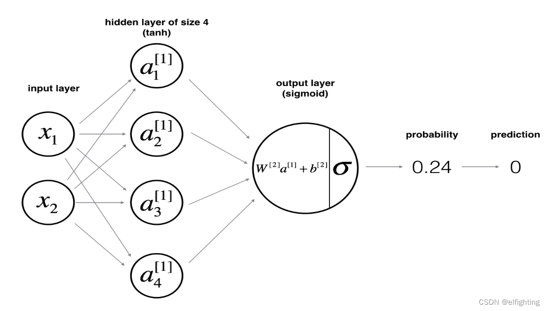
         1. 基本结构定义

# GRADED FUNCTION: layer_sizes

def layer_sizes(X, Y):
    """
    Arguments:
    X -- input dataset of shape (input size, number of examples)
    Y -- labels of shape (output size, number of examples)
    
    Returns:
    n_x -- the size of the input layer
    n_h -- the size of the hidden layer
    n_y -- the size of the output layer
    """
   
    # YOUR CODE STARTS HERE
    n_x = X.shape[0]
    n_h = 4
    n_y = Y.shape[0]
    
    # YOUR CODE ENDS HERE
    return (n_x, n_h, n_y)

           注意，n_x和n_y 是由数据集决定的，而n_h即hidden layer中neuron的数量则是可以自由选择的，此处我们定义为4。

        2. 参数初始化

        利用 np.random.randn(a,b) 对参数W进行随机初始化，而b不是matrix而是vector，朱姐用np.zeros((a,b))初始化成0即可。注意每一个layer都有自己的参数W和b：

# GRADED FUNCTION: initialize_parameters

def initialize_parameters(n_x, n_h, n_y):
    """
    Argument:
    n_x -- size of the input layer
    n_h -- size of the hidden layer
    n_y -- size of the output layer
    
    Returns:
    params -- python dictionary containing your parameters:
                    W1 -- weight matrix of shape (n_h, n_x)
                    b1 -- bias vector of shape (n_h, 1)
                    W2 -- weight matrix of shape (n_y, n_h)
                    b2 -- bias vector of shape (n_y, 1)
    """    
    # YOUR CODE STARTS HERE
    W1 = np.random.randn(n_h, n_x) * 0.01
    b1 = np.zeros((n_h, 1))
    W2 = np.random.randn(n_y, n_h) * 0.01
    b2 = np.zeros((n_y, 1))
    
    # YOUR CODE ENDS HERE

    parameters = {"W1": W1,
                  "b1": b1,
                  "W2": W2,
                  "b2": b2}
    
    return parameters

        3. forward propagtion        

# GRADED FUNCTION:forward_propagation

def forward_propagation(X, parameters):
    """
    Argument:
    X -- input data of size (n_x, m)
    parameters -- python dictionary containing your parameters (output of initialization function)
    
    Returns:
    A2 -- The sigmoid output of the second activation
    cache -- a dictionary containing "Z1", "A1", "Z2" and "A2"
    """
    # Retrieve each parameter from the dictionary "parameters"
    #(≈ 4 lines of code)
    # YOUR CODE STARTS HERE
    W1 = parameters["W1"]
    b1 = parameters["b1"]
    W2 = parameters["W2"]
    b2 = parameters["b2"]
    
    # YOUR CODE ENDS HERE
    
    # Implement Forward Propagation to calculate A2 (probabilities)
    # (≈ 4 lines of code)
    # YOUR CODE STARTS HERE
    Z1 = np.dot(W1, X)+b1
    A1 = np.tanh(Z1)
    Z2 = np.dot(W2, A1)+b2
    A2 = sigmoid(Z2)
    
    # YOUR CODE ENDS HERE
    
    assert(A2.shape == (1, X.shape[1]))
    
    cache = {"Z1": Z1,
             "A1": A1,
             "Z2": Z2,
             "A2": A2}
    
    return A2, cache

        4. Compute the cost

# GRADED FUNCTION: compute_cost

def compute_cost(A2, Y):
    """
    Computes the cross-entropy cost given in equation (13)
    
    Arguments:
    A2 -- The sigmoid output of the second activation, of shape (1, number of examples)
    Y -- "true" labels vector of shape (1, number of examples)

    Returns:
    cost -- cross-entropy cost given equation (13)
    
    """
    
    m = Y.shape[1] # number of examples

    # Compute the cross-entropy cost
    # (≈ 2 lines of code)
    # YOUR CODE STARTS HERE
    cost = np.dot(Y, np.log(A2.T))+np.dot(1-Y, np.log(1-A2.T))
    cost = -cost/m
    
    # YOUR CODE ENDS HERE
    
    cost = float(np.squeeze(cost))  # makes sure cost is the dimension we expect. 
                                    # E.g., turns [[17]] into 17 
    
    return cost

        5. Backpropagation

# GRADED FUNCTION: backward_propagation

def backward_propagation(parameters, cache, X, Y):
    """
    Implement the backward propagation using the instructions above.
    
    Arguments:
    parameters -- python dictionary containing our parameters 
    cache -- a dictionary containing "Z1", "A1", "Z2" and "A2".
    X -- input data of shape (2, number of examples)
    Y -- "true" labels vector of shape (1, number of examples)
    
    Returns:
    grads -- python dictionary containing your gradients with respect to different parameters
    """
    m = X.shape[1]
    
    # First, retrieve W1 and W2 from the dictionary "parameters".
    #(≈ 2 lines of code)
    # YOUR CODE STARTS HERE
    W1 = parameters["W1"]
    W2 = parameters["W2"]
    
    # YOUR CODE ENDS HERE
        
    # Retrieve also A1 and A2 from dictionary "cache".
    #(≈ 2 lines of code)
    # YOUR CODE STARTS HERE
    A1 = cache["A1"]
    A2 = cache["A2"]
    
    # YOUR CODE ENDS HERE
    
    # Backward propagation: calculate dW1, db1, dW2, db2. 
    #(≈ 6 lines of code, corresponding to 6 equations on slide above)
    # YOUR CODE STARTS HERE
    dZ2 = A2 - Y # (n, m)
    dW2 = np.dot(dZ2, A1.T)/m # (n,m)*(m,n_h)=(n,n_h)
    db2 = np.sum(dZ2, axis = 1,keepdims = True)/m # (n_h, 1)
    dZ1 = np.dot(W2.T, dZ2)*(1-np.power(A1,2))
    dW1 = np.dot(dZ1, X.T)/m
    db1 = np.sum(dZ1, axis = 1,keepdims=True)/m
    
    
    # YOUR CODE ENDS HERE
    
    grads = {"dW1": dW1,
             "db1": db1,
             "dW2": dW2,
             "db2": db2}
    
    return grads

        6. Update Parameters

# GRADED FUNCTION: update_parameters

def update_parameters(parameters, grads, learning_rate = 1.2):
    """
    Updates parameters using the gradient descent update rule given above
    
    Arguments:
    parameters -- python dictionary containing your parameters 
    grads -- python dictionary containing your gradients 
    
    Returns:
    parameters -- python dictionary containing your updated parameters 
    """
    # Retrieve a copy of each parameter from the dictionary "parameters". Use copy.deepcopy(...) for W1 and W2
    #(≈ 4 lines of code)
    # YOUR CODE STARTS HERE
    W1 = parameters["W1"]
    b1 = parameters["b1"]
    W2 = parameters["W2"]
    b2 = parameters["b2"]
    
    # YOUR CODE ENDS HERE
    
    # Retrieve each gradient from the dictionary "grads"
    #(≈ 4 lines of code)
    # YOUR CODE STARTS HERE
    dW1 = grads["dW1"]
    db1 = grads["db1"]
    dW2 = grads["dW2"]
    db2 = grads["db2"]
    
    # YOUR CODE ENDS HERE
    
    # Update rule for each parameter
    #(≈ 4 lines of code)
    # YOUR CODE STARTS HERE
    W1 = W1 - learning_rate*dW1
    b1 = b1 - learning_rate*db1
    W2 = W2 - learning_rate*dW2
    b2 = b2 - learning_rate*db2
    
    # YOUR CODE ENDS HERE
    
    parameters = {"W1": W1,
                  "b1": b1,
                  "W2": W2,
                  "b2": b2}
    
    return parameters

        6. Integration

# GRADED FUNCTION: nn_model

def nn_model(X, Y, n_h, num_iterations = 10000, print_cost=False):
    """
    Arguments:
    X -- dataset of shape (2, number of examples)
    Y -- labels of shape (1, number of examples)
    n_h -- size of the hidden layer
    num_iterations -- Number of iterations in gradient descent loop
    print_cost -- if True, print the cost every 1000 iterations
    
    Returns:
    parameters -- parameters learnt by the model. They can then be used to predict.
    """
    
    np.random.seed(3)
    n_x = layer_sizes(X, Y)[0]
    n_y = layer_sizes(X, Y)[2]
    
    # Initialize parameters
    #(≈ 1 line of code)
    # YOUR CODE STARTS HERE
    parameters = initialize_parameters(n_x, n_h, n_y)
    
    # YOUR CODE ENDS HERE
    
    # Loop (gradient descent)

    for i in range(0, num_iterations):
         
        # YOUR CODE STARTS HERE
        
        #(≈ 4 lines of code)
        # Forward propagation. Inputs: "X, parameters". Outputs: "A2, cache".
        A2, cache = forward_propagation(X, parameters)
        
        # Cost function. Inputs: "A2, Y". Outputs: "cost".
        cost = compute_cost(A2, Y)
 
        # Backpropagation. Inputs: "parameters, cache, X, Y". Outputs: "grads".
        grads = backward_propagation(parameters, cache, X, Y)
 
        # Gradient descent parameter update. Inputs: "parameters, grads". Outputs: "parameters".
        parameters = update_parameters(parameters, grads)
        
        
        
        # YOUR CODE ENDS HERE
        
        # Print the cost every 1000 iterations
        if print_cost and i % 1000 == 0:
            print ("Cost after iteration %i: %f" %(i, cost))

    return parameters

四、Test the Model

        1. Predict

# GRADED FUNCTION: predict

def predict(parameters, X):
    """
    Using the learned parameters, predicts a class for each example in X
    
    Arguments:
    parameters -- python dictionary containing your parameters 
    X -- input data of size (n_x, m)
    
    Returns
    predictions -- vector of predictions of our model (red: 0 / blue: 1)
    """
    
    # Computes probabilities using forward propagation, and classifies to 0/1 using 0.5 as the threshold.
    #(≈ 2 lines of code)
    # YOUR CODE STARTS HERE
    A2, cache = forward_propagation(X, parameters)
    predictions = (A2>0.5)
    
    # YOUR CODE ENDS HERE
    
    return predictions

        2. Test the Model

# Print accuracy
predictions = predict(parameters, X)
print ('Accuracy: %d' % float((np.dot(Y, predictions.T) + np.dot(1 - Y, 1 - predictions.T)) / float(Y.size) * 100) + '%')

        最终得到的准确率为90%。并且根据实验，适当增加hidden units的数量可以提高准确率