R语言做聚类分析Kmeans时确定类的个数

最新推荐文章于 2024-05-20 20:30:21 发布

faith默默

最新推荐文章于 2024-05-20 20:30:21 发布

阅读量2.8w

点赞数 9

分类专栏： R 文章标签： r语言

R 专栏收录该内容

50 篇文章 4 订阅

订阅专栏

方法一：

K平均算法（k-means）
在下面的误差平方和图中，拐点（bend or elbow）的位置对应的x轴即k-means聚类给出的合适的类的个数。

> n = 100
> g=6
> set.seed(g)
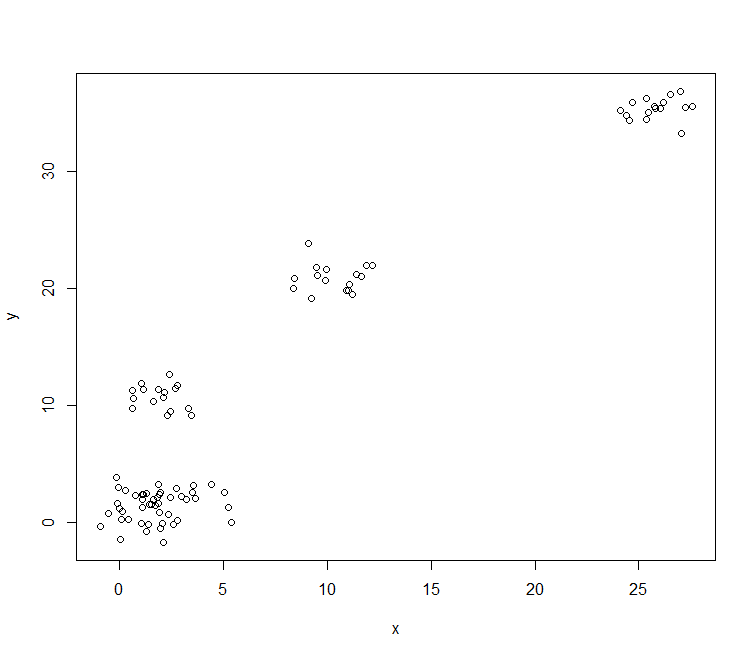
> d <- data.frame(x = unlist(lapply(1:g, function(i) rnorm(n/g, runif(1)*i^2))), y = unlist(lapply(1:g, function(i) rnorm(n/g, runif(1)*i^2))))
> plot(d)
>

这里写图片描述

> mydata <- d
> 
> wss <- (nrow(mydata)-1)*sum(apply(mydata,2,var))
> for (i in 2:15)
+ wss[i] <- sum(kmeans(mydata,centers=i)$withinss)
> ###这里的wss(within-cluster sum of squares)是组内平方和
> plot(1:15, wss, type="b", xlab="Number of Clusters",ylab="Within groups sum of squares")
>

这里写图片描述
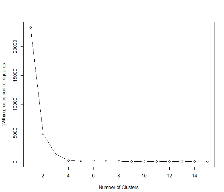
由上图可以看出，该方法给出合理的类别个数是4个。

方法二：

K中心聚类算法（K-mediods）
使用fpc包里的pamk函数来估计类的个数：

> library(cluster)
Warning message:
程辑包‘cluster’是用R版本3.2.3 来建造的 
> library(fpc)
> pamk.best <- pamk(d)
> cat("number of clusters estimated by optimum average silhouette width:", pamk.best$nc, "\n") 
number of clusters estimated by optimum average silhouette width: 4 
> plot(pam(d, pamk.best$nc))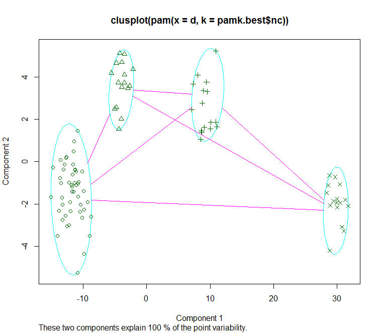

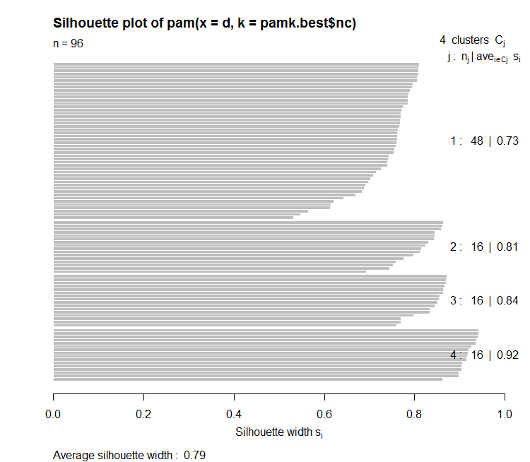
这里写图片描述

sihouette值是用来表示某一个对象和它所属类的凝合力强度以及和其他类分离强度的，值范围为-1到1，值越大表示该对象越匹配所属类以及和邻近类有多不匹配。
所以从上图sihouette plot中可以看出，该方法给出的合理类的个数为4个。

方法三：

基于Calinsky Criterion

> require(vegan)
载入需要的程辑包：vegan
载入需要的程辑包：permute
载入需要的程辑包：lattice
This is vegan 2.4-0
Warning messages:
1: 程辑包‘vegan’是用R版本3.2.5 来建造的 
2: 程辑包‘permute’是用R版本3.2.5 来建造的 
3: 程辑包‘lattice’是用R版本3.2.3 来建造的 
> fit <- cascadeKM(scale(d, center = TRUE,  scale = TRUE), 1, 10, iter = 1000)
> plot(fit, sortg = TRUE, grpmts.plot = TRUE)
> calinski.best <- as.numeric(which.max(fit$results[2,]))
> cat("Calinski criterion optimal number of clusters:", calinski.best, "\n")
Calinski criterion optimal number of clusters: 5 
>

这里写图片描述

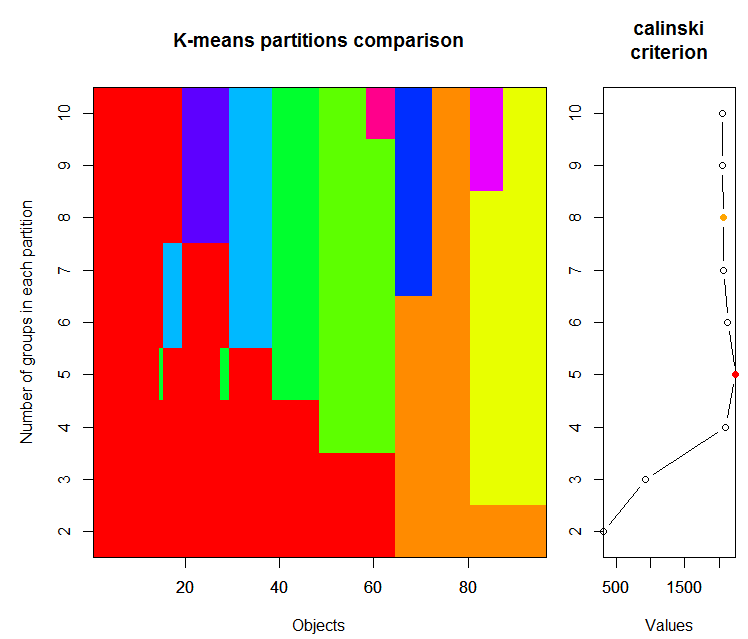
由上图我们可以看到，根据Calinsky标准，得到类的个数是5个。

方法四：

基于模型假设的聚类，利用的是mclust包：

> library(mclust)
    __  ___________    __  _____________
   /  |/  / ____/ /   / / / / ___/_  __/
  / /|_/ / /   / /   / / / /\__ \ / /   
 / /  / / /___/ /___/ /_/ /___/ // /    
/_/  /_/\____/_____/\____//____//_/    version 5.1
Type 'citation("mclust")' for citing this R package in publications.
Warning message:
程辑包‘mclust’是用R版本3.2.4 来建造的 
> d_clust <- Mclust(as.matrix(d), G=1:20)
> m.best <- dim(d_clust$z)[2]
> cat("model-based optimal number of clusters:", m.best, "\n")
model-based optimal number of clusters: 4 
> plot(d_clust)
Model-based clustering plots: 

1: BIC
2: classification
3: uncertainty
4: density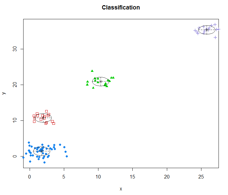

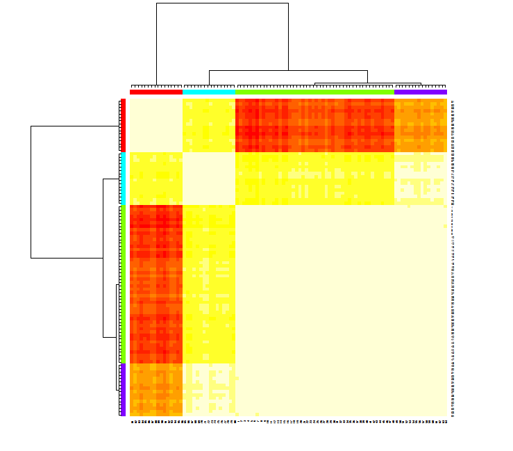
这里写图片描述

方法五：

基于AP算法的聚类

> library(apcluster) 

载入程辑包：‘apcluster’

The following object is masked from ‘package:stats’:

    heatmap

Warning message:
程辑包‘apcluster’是用R版本3.2.5 来建造的 
> d.apclus <- apcluster(negDistMat(r=2), d) 
> cat("affinity propogation optimal number of clusters:", length(d.apclus@clusters), "\n") 
affinity propogation optimal number of clusters: 4 
> #4 得出的分类个数 
> heatmap(d.apclus) 
> plot(d.apclus, d)
>