


文章来源于机器学习算法与Python实战,作者奥辰
TensorFlow2.0(6):利用data模块进行数据预处理
TensorFlow2.0(9):神器级可视化工具TensorBoard
TensorFlow2.0(10):加载自定义图片数据集到Dataset
TensorFlow2.0(11):tf.keras建模三部曲
TensorFlow2.0(1):基本数据结构——张量
1.1引言
TensorFlow2.0版本已经发布,虽然不是正式版,但预览版都发布了,正式版还会远吗?相比于1.X,2.0版的TensorFlow修改的不是一点半点,这些修改极大的弥补了1.X版本的反人类设计,提升了框架的整体易用性,绝对好评!
赶紧来学习一波吧,做最先吃螃蟹的那一批人!先从TensorFlow的基本数据结构——张量(tensor)开始。
1.2 创建
1.2.1 constant()方法
import tensorflow as tf
tf.constant(1) # 创建一个整型张量
<tf.Tensor: id=0, shape=(), dtype=int32, numpy=1>
tf.constant(1.) # 创建一个浮点型张量
<tf.Tensor: id=2, shape=(), dtype=float32, numpy=1.0>
tf.constant(2., dtype=tf.double) # 创建的同时指定数据类型
<tf.Tensor: id=4, shape=(), dtype=float64, numpy=2.0>
tf.constant([[1.,2.,3.],[4.,5.,6.]]) # 通过传入一个list参数创建
<tf.Tensor: id=6, shape=(2, 3), dtype=float32, numpy=
array([[1., 2., 3.],
       [4., 5., 6.]], dtype=float32)>
如果输入的数据与指定的数据类型不相符,会产生以下异常:
TypeError: Cannot convert provided value to EagerTensor. Provided value: 2.1 Requested dtype: int32
1.2.2 convert_to_tensor()方法
import numpy as np
tf.convert_to_tensor(np.ones([2, 3]))
<tf.Tensor: id=9, shape=(2, 3), dtype=float64, numpy=
array([[1., 1., 1.],
       [1., 1., 1.]])>
tf.convert_to_tensor(np.ones([2, 3]))
<tf.Tensor: id=11, shape=(2, 3), dtype=float64, numpy=
array([[1., 1., 1.],
       [1., 1., 1.]])>
tf.convert_to_tensor([[2.,3.],[3., 4.]])
<tf.Tensor: id=13, shape=(2, 2), dtype=float32, numpy=
array([[2., 3.],
       [3., 4.]], dtype=float32)>
1.2.3 创建元素为指定值的tensor
如果你熟悉numpy创建数组的方法,你一定见过zeros()、ones()等方法,TensorFlow中也有这些方法。
(1)zeros()与ones()
a = tf.zeros([2, 3, 3]) # 创建一个元素全为0,形状为[2, 3, 3]的tensor
a
<tf.Tensor: id=46, shape=(2, 3, 3), dtype=float32, numpy=
array([[[0., 0., 0.],
        [0., 0., 0.],
        [0., 0., 0.]],

       [[0., 0., 0.],
        [0., 0., 0.],
        [0., 0., 0.]]], dtype=float32)>
b = tf.ones([2, 3]) # 创建一个元素全为1,形状为[2, 3]的tensor
b
<tf.Tensor: id=50, shape=(2, 3), dtype=float32, numpy=
array([[1., 1., 1.],
       [1., 1., 1.]], dtype=float32)>
(2)zeros_like()与ones_like
tf.zeros_like(b) # 仿照b的shape创建一个全为0的tensor
<tf.Tensor: id=52, shape=(2, 3), dtype=float32, numpy=
array([[0., 0., 0.],
       [0., 0., 0.]], dtype=float32)>
tf.ones_like(a) # 仿照b的shape创建一个全为1的tensor
<tf.Tensor: id=56, shape=(2, 3, 3), dtype=float32, numpy=
array([[[1., 1., 1.],
        [1., 1., 1.],
        [1., 1., 1.]],

       [[1., 1., 1.],
        [1., 1., 1.],
        [1., 1., 1.]]], dtype=float32)>
(3)fill()
tf.fill([2,3],5) # 创建元素全为5,形状为[2,3]的tensor
<tf.Tensor: id=38, shape=(2, 3), dtype=int32, numpy=
array([[5, 5, 5],
       [5, 5, 5]])>
1.2.4 随机初始化
在实际应用中,经常需要随机初始化元素服从某种分布的tensor,TensorFlow中也提供了这种功能。
**(1)从指定正态分布中随机取值:tf.random.normal()。**例如,随机初始化一个元素服从均值为1,方差为1的正态分布且形状为[2, 3]的tensor:
tf.random.normal([2, 3], mean=1, stddev=1)
<tf.Tensor: id=63, shape=(2, 3), dtype=float32, numpy=
array([[ 1.7034731 ,  0.4979009 ,  1.4266468 ],
       [-0.33414853,  0.2618034 ,  0.3966313 ]], dtype=float32)>
**(2)从指定的截断正态分布中随机取值:truncated_normal()。**意思是从指定的正太分布中取值,但是取值范围在两个标准差范围内,也就是:[ mean - 2 * stddev, mean + 2 * stddev ]
tf.random.truncated_normal([2, 3], mean=1, stddev=1)
<tf.Tensor: id=70, shape=(2, 3), dtype=float32, numpy=
array([[0.71736836, 1.7930655 , 0.47575486],
       [0.83504593, 0.7969478 , 0.6002228 ]], dtype=float32)>
(3)从指定均匀分布中随机取值:tf.random.uniform()。
tf.random.uniform([2, 3], minval=1, maxval=2) # 在1~2之间均匀分布
<tf.Tensor: id=78, shape=(2, 3), dtype=float32, numpy=
array([[1.7117869, 1.2625391, 1.6652637],
       [1.3810604, 1.0297629, 1.1268978]], dtype=float32)>
1.3 索引
a = tf.convert_to_tensor(np.arange(80).reshape(2,2,4,5))
a
<tf.Tensor: id=80, shape=(2, 2, 4, 5), dtype=int32, numpy=
array([[[[ 0,  1,  2,  3,  4],
         [ 5,  6,  7,  8,  9],
         [10, 11, 12, 13, 14],
         [15, 16, 17, 18, 19]],

        [[20, 21, 22, 23, 24],
         [25, 26, 27, 28, 29],
         [30, 31, 32, 33, 34],
         [35, 36, 37, 38, 39]]],


       [[[40, 41, 42, 43, 44],
         [45, 46, 47, 48, 49],
         [50, 51, 52, 53, 54],
         [55, 56, 57, 58, 59]],

        [[60, 61, 62, 63, 64],
         [65, 66, 67, 68, 69],
         [70, 71, 72, 73, 74],
         [75, 76, 77, 78, 79]]]])>
1.3.1 基础索引
TensorFlow支持Python原生的基础索引方式,即多个方括号逐步索引取值:[idx][idx][idx],每个方括号对应一个维度。
a[0] # 取第一个维度
<tf.Tensor: id=85, shape=(2, 4, 5), dtype=int32, numpy=
array([[[ 0,  1,  2,  3,  4],
        [ 5,  6,  7,  8,  9],
        [10, 11, 12, 13, 14],
        [15, 16, 17, 18, 19]],

       [[20, 21, 22, 23, 24],
        [25, 26, 27, 28, 29],
        [30, 31, 32, 33, 34],
        [35, 36, 37, 38, 39]]])>
a[0][1] # 同时筛选两个维度
<tf.Tensor: id=94, shape=(4, 5), dtype=int32, numpy=
array([[20, 21, 22, 23, 24],
       [25, 26, 27, 28, 29],
       [30, 31, 32, 33, 34],
       [35, 36, 37, 38, 39]])>
a[0][1][3][3] # 同时对4个维度进行筛选
<tf.Tensor: id=111, shape=(), dtype=int32, numpy=38>
这种索引数据的方法简单,易于理解,但是可读性差,只能按维度依次索引数据,也不能索引列。
1.3.2 numpy索引
TensorFlow也继承了numpy中的部分索引方式,如果对numpy索引方式不熟悉,可以查看我的前几篇博客。
(1)[idx1, idx2, idx3]
这种索引方式是在一个方括号内写下所有的索引,每个索引序号之间用逗号隔开。
a[1] # 筛选第一维度,这跟基础索引一样
<tf.Tensor: id=116, shape=(2, 4, 5), dtype=int32, numpy=
array([[[40, 41, 42, 43, 44],
        [45, 46, 47, 48, 49],
        [50, 51, 52, 53, 54],
        [55, 56, 57, 58, 59]],

       [[60, 61, 62, 63, 64],
        [65, 66, 67, 68, 69],
        [70, 71, 72, 73, 74],
        [75, 76, 77, 78, 79]]])>
a[1,1, 3] # 同时帅选3个维度
<tf.Tensor: id=121, shape=(5,), dtype=int32, numpy=array([75, 76, 77, 78, 79])>
(2)冒号切片与步长:[start:end:step]
这种索引方式在Python原生的list类型中也是常见的,而且使用方法也是一样的。
a[1,:,0:2] # 对第1维度选第二块数据,对第二维度选所有数据,对第三维度选前两行
<tf.Tensor: id=126, shape=(2, 2, 5), dtype=int32, numpy=
array([[[40, 41, 42, 43, 44],
        [45, 46, 47, 48, 49]],

       [[60, 61, 62, 63, 64],
        [65, 66, 67, 68, 69]]])>
a[1,:,0:2,0:4] # 继续上面的例子,对第4维度筛选去前4列
<tf.Tensor: id=131, shape=(2, 2, 4), dtype=int32, numpy=
array([[[40, 41, 42, 43],
        [45, 46, 47, 48]],

       [[60, 61, 62, 63],
        [65, 66, 67, 68]]])>
a[1,:,0:2,0:4:2] # 对第4维度加上步长,每隔一个数据取一次
<tf.Tensor: id=136, shape=(2, 2, 2), dtype=int32, numpy=
array([[[40, 42],
        [45, 47]],

       [[60, 62],
        [65, 67]]])>
也可以使用负值步长表示逆序索引,但要注意,负数步长时,原本的[start : end : step]也要跟着编程[end : start : step]:
a[1,:,0:2,4:0:-1]
<tf.Tensor: id=141, shape=(2, 2, 4), dtype=int32, numpy=
array([[[44, 43, 42, 41],
        [49, 48, 47, 46]],

       [[64, 63, 62, 61],
        [69, 68, 67, 66]]])>
a[1,:,0:2,4:0:-2]
<tf.Tensor: id=146, shape=(2, 2, 2), dtype=int32, numpy=
array([[[44, 42],
        [49, 47]],

       [[64, 62],
        [69, 67]]])>
在numpy和TensorFlow中还有“..."(三个英文句号)的使用,“..."用于表示连续多个维度全选:
a[1,...,0:4] # 等同于a[1, : , : ,0:4]
<tf.Tensor: id=151, shape=(2, 4, 4), dtype=int32, numpy=
array([[[40, 41, 42, 43],
        [45, 46, 47, 48],
        [50, 51, 52, 53],
        [55, 56, 57, 58]],

       [[60, 61, 62, 63],
        [65, 66, 67, 68],
        [70, 71, 72, 73],
        [75, 76, 77, 78]]])>
a[0,0,...] # 等同于a[0,0,:,:]
<tf.Tensor: id=156, shape=(4, 5), dtype=int32, numpy=
array([[ 0,  1,  2,  3,  4],
       [ 5,  6,  7,  8,  9],
       [10, 11, 12, 13, 14],
       [15, 16, 17, 18, 19]])>
1.3.3 gather与gather_nd
gather与gather_nd是指TensorFlow通过gather()方法和gather_nd()方法提供的两种索引方式。在numpy中,可以通过嵌套list的方式来指定无规则的索引:
b = np.arange(20).reshape(4,5)
b[1, [0,3,4]] # 选取第2行的第1列、第4列、第5列
array([5, 8, 9])
但是在TensorFlow中,这种索引方式并没有从numpy中继承下来,所以如果在Tensor中使用这种方式,会抛出以下异常:
TypeError: Only integers, slices (:), ellipsis (...), tf.newaxis (None) and scalar tf.int32/tf.int64 tensors are valid indices, got [0, 3, 4]
还好的是,在TensorFlow中通过gather()方法和gather_nd()方法提供了这种索引方法。
(1)gather()方法
tf.gather(b, axis=0, indices=[0, 2, 3]) # 选取第1行,第3行,第4行
<tf.Tensor: id=163, shape=(3, 5), dtype=int32, numpy=
array([[ 0,  1,  2,  3,  4],
       [10, 11, 12, 13, 14],
       [15, 16, 17, 18, 19]])>
tf.gather(b, axis=1, indices=[0, 2, 3]) # 选取第1列,第3列,第4列
<tf.Tensor: id=168, shape=(4, 3), dtype=int32, numpy=
array([[ 0,  2,  3],
       [ 5,  7,  8],
       [10, 12, 13],
       [15, 17, 18]])>
仔细观察上面gather()方法例子,可以发现,第一个参数时数据源,还有两个参数中,axis指的是将要的维度,indices指的是需要选取的序号。
(2)gather_nd()
gather()方法一次只能对一个维度进行索引,gather_nd()方法可以同时对多个维度进行索引。
tf.gather_nd(b, [[0, 2],[3, 3]]) # 选取第1行第3列的那个数据,和第4行第4列的数据
<tf.Tensor: id=172, shape=(2,), dtype=int32, numpy=array([ 2, 18])>
1.3.5 条件索引
可以结合一些简单的逻辑运算符进行索引取值:
import tensorflow as tf
a = tf.random.uniform([3,3],minval=-10,maxval=10,dtype=tf.int32)
a
<tf.Tensor: id=17, shape=(3, 3), dtype=int32, numpy=
array([[-7, -9,  6],
       [-6, -5,  9],
       [ 8,  9,  4]])>
mask = a < 0
mask
<tf.Tensor: id=20, shape=(3, 3), dtype=bool, numpy=
array([[ True,  True, False],
       [ True,  True, False],
       [False, False, False]])>
可以看到,返回的是一个shape与a相同的tensor,在a小于零的位置是True,大于零的位置为False。进一步地,我们可以用boolwan_mask()方法直接取出符合条件的元素:
tf.boolean_mask(a,mask)
<tf.Tensor: id=82, shape=(4,), dtype=int32, numpy=array([-7, -9, -6, -5])>
可以结合where()方法取出符合条件元素的索引:
m_index = tf.where(mask)
m_index
<tf.Tensor: id=84, shape=(4, 2), dtype=int64, numpy=
array([[0, 0],
       [0, 1],
       [1, 0],
       [1, 1]], dtype=int64)>
再使用之前说过的gather_nd()方法取值:
tf.gather_nd(a,m_index)
<tf.Tensor: id=86, shape=(4,), dtype=int32, numpy=array([-7, -9, -6, -5])>
where()方法还有第二种用法——从两个tensor中取出符合条件的值,这时候where()方法必须接受3个参数:
condition = tf.random.uniform([3,3],minval=0,maxval=2,dtype=tf.int32)
condition = tf.cast(condition, tf.bool)
condition
<tf.Tensor: id=124, shape=(3, 3), dtype=bool, numpy=
array([[ True,  True, False],
       [ True, False, False],
       [ True, False, False]])>
a = tf.range(1,10)
a = tf.reshape(a,[3,3])
a
<tf.Tensor: id=162, shape=(3, 3), dtype=int32, numpy=
array([[1, 2, 3],
       [4, 5, 6],
       [7, 8, 9]])>
b = tf.range(-9,0)
b = tf.reshape(b,[3,3])
b
<tf.Tensor: id=169, shape=(3, 3), dtype=int32, numpy=
array([[-9, -8, -7],
       [-6, -5, -4],
       [-3, -2, -1]])>
tf.where(condition, a, b)
<tf.Tensor: id=171, shape=(3, 3), dtype=int32, numpy=
array([[ 1,  2, -7],
       [ 4, -5, -4],
       [ 7, -2, -1]])>
上面where()方法返回的结果在True的位置取值是a中对应位置元素的值,在False位置是b中对应元素的值。
1.4 维度变换
1.4.1 reshape()
numpy中的ndarray数组有个一reshape()方法,用来改变数组的shape,TensorFlow中的reshape()方法,功能也是一样的,不过TensorFlow中的reshape()没有绑定到tensor中:
a = tf.ones([2,3,4])
a.shape
TensorShape([2, 3, 4])
a
<tf.Tensor: id=176, shape=(2, 3, 4), dtype=float32, numpy=
array([[[1., 1., 1., 1.],
        [1., 1., 1., 1.],
        [1., 1., 1., 1.]],

       [[1., 1., 1., 1.],
        [1., 1., 1., 1.],
        [1., 1., 1., 1.]]], dtype=float32)>
b = tf.reshape(a, [2, 2, 6])
b.shape
TensorShape([2, 2, 6])
b
<tf.Tensor: id=179, shape=(2, 2, 6), dtype=float32, numpy=
array([[[1., 1., 1., 1., 1., 1.],
        [1., 1., 1., 1., 1., 1.]],

       [[1., 1., 1., 1., 1., 1.],
        [1., 1., 1., 1., 1., 1.]]], dtype=float32)>
c = tf.reshape(a, [3, 2, 4])
c
<tf.Tensor: id=183, shape=(3, 2, 4), dtype=float32, numpy=
array([[[1., 1., 1., 1.],
        [1., 1., 1., 1.]],

       [[1., 1., 1., 1.],
        [1., 1., 1., 1.]],

       [[1., 1., 1., 1.],
        [1., 1., 1., 1.]]], dtype=float32)>
可以看到,在上面的例子中,通过reshape()方法可以很方便的改变tensor的形状,得到一个新的tensor,需要注意的是在进行维度变换时,数据的重量是不变的,上面的例子无论是[2,3,4], [2, 2, 6]还是[3, 2, 4]都对应总量24,如果对应不上,就会产生异常。
1.4.2 转置:transpose()
transpose()方法提供了一种类似于装置的操作:
a = tf.constant([[1,2,3],[4,5,6]])
a.shape
TensorShape([2, 3])
b = tf.transpose(a)
b.shape
TensorShape([3, 2])
b
<tf.Tensor: id=192, shape=(3, 2), dtype=int32, numpy=
array([[1, 4],
       [2, 5],
       [3, 6]])>
在默认情况下,transpose()方法会将所有维度按逆序方式完全转置,当然也可以通过perm参数执行需要转置的维度:
a=tf.constant([[[1,2,3],[4,5,6]],[[7,8,9],[10,11,12]]])
a
<tf.Tensor: id=194, shape=(2, 2, 3), dtype=int32, numpy=
array([[[ 1,  2,  3],
        [ 4,  5,  6]],

       [[ 7,  8,  9],
        [10, 11, 12]]])>
b = tf.transpose(a) # 不指定perm参数时,相当于tf.transpose(a, perm=[2, 1, 0])
b
<tf.Tensor: id=197, shape=(3, 2, 2), dtype=int32, numpy=
array([[[ 1,  7],
        [ 4, 10]],

       [[ 2,  8],
        [ 5, 11]],

       [[ 3,  9],
        [ 6, 12]]])>
c = tf.transpose(a, perm=[2, 1, 0])
c
<tf.Tensor: id=200, shape=(3, 2, 2), dtype=int32, numpy=
array([[[ 1,  7],
        [ 4, 10]],

       [[ 2,  8],
        [ 5, 11]],

       [[ 3,  9],
        [ 6, 12]]])>
d = tf.transpose(a, perm=[0, 2, 1]) # 第一个维度不做变换,对第二、第三维度进行转置
d
<tf.Tensor: id=203, shape=(2, 3, 2), dtype=int32, numpy=
array([[[ 1,  4],
        [ 2,  5],
        [ 3,  6]],

       [[ 7, 10],
        [ 8, 11],
        [ 9, 12]]])>
1.4.3 添加维度:expand_dims()
a=tf.constant([[1,2,3],[4,5,6]])
a
<tf.Tensor: id=205, shape=(2, 3), dtype=int32, numpy=
array([[1, 2, 3],
       [4, 5, 6]])>
tf.expand_dims(a, axis=0)
<tf.Tensor: id=208, shape=(1, 2, 3), dtype=int32, numpy=
array([[[1, 2, 3],
        [4, 5, 6]]])>
tf.expand_dims(a, axis=1)
<tf.Tensor: id=211, shape=(2, 1, 3), dtype=int32, numpy=
array([[[1, 2, 3]],

       [[4, 5, 6]]])>
tf.expand_dims(a, axis=-1)
<tf.Tensor: id=214, shape=(2, 3, 1), dtype=int32, numpy=
array([[[1],
        [2],
        [3]],

       [[4],
        [5],
        [6]]])>
tf.expand_dims(a, axis=2)
<tf.Tensor: id=217, shape=(2, 3, 1), dtype=int32, numpy=
array([[[1],
        [2],
        [3]],

       [[4],
        [5],
        [6]]])>
expand_dims()方法添加维度时,通过axis参数指定添加维度的位置,正数表示从前往后数,负数表示从后往前数。
1.4.4 压缩维度:squeeze()
squeeze()方法与expand_dims()方法作用刚好相反,其作用是删除张量中dim为1的维度:
a = tf.ones([1,3,1,2])
a
<tf.Tensor: id=221, shape=(1, 3, 1, 2), dtype=float32, numpy=
array([[[[1., 1.]],

        [[1., 1.]],

        [[1., 1.]]]], dtype=float32)>
tf.squeeze(a)
<tf.Tensor: id=223, shape=(3, 2), dtype=float32, numpy=
array([[1., 1.],
       [1., 1.],
       [1., 1.]], dtype=float32)>
TensorFlow2.0(2):数学运算
2.1 基本运算:(+、-、*、/、//、%)
基本运算中所有实例都以下面的张量a、b为例进行:
import tensorflow as tf
a = tf.random.uniform([2, 3], minval=1, maxval=6,dtype=tf.int32)
b = tf.random.uniform([2, 3], minval=1, maxval=6,dtype=tf.int32)
a
<tf.Tensor: id=3, shape=(2, 3), dtype=int32, numpy=
array([[1, 4, 5],
       [5, 1, 4]])>
b
<tf.Tensor: id=7, shape=(2, 3), dtype=int32, numpy=
array([[1, 3, 5],
       [3, 5, 2]])>
(1)加(+)
tf.add(a,b) # 通过add方法执行加操作
<tf.Tensor: id=12, shape=(2, 3), dtype=int32, numpy=
array([[ 2,  7, 10],
       [ 8,  6,  6]])>
a + b # 也可以通过操作符进行
<tf.Tensor: id=16, shape=(2, 3), dtype=int32, numpy=
array([[ 2,  7, 10],
       [ 8,  6,  6]])>
(2)减(-)
tf.subtract(a,b)
<tf.Tensor: id=18, shape=(2, 3), dtype=int32, numpy=
array([[ 0,  1,  0],
       [ 2, -4,  2]])>
a - b
<tf.Tensor: id=20, shape=(2, 3), dtype=int32, numpy=
array([[ 0,  1,  0],
       [ 2, -4,  2]])>
(3)乘法(*)
tf.multiply(a,b)
<tf.Tensor: id=22, shape=(2, 3), dtype=int32, numpy=
array([[ 1, 12, 25],
       [15,  5,  8]])>
a * b
<tf.Tensor: id=24, shape=(2, 3), dtype=int32, numpy=
array([[ 1, 12, 25],
       [15,  5,  8]])>
(4)除法(/)
tf.divide(a,b)
<tf.Tensor: id=28, shape=(2, 3), dtype=float64, numpy=
array([[1.        , 1.33333333, 1.        ],
       [1.66666667, 0.2       , 2.        ]])>
a/b
<tf.Tensor: id=32, shape=(2, 3), dtype=float64, numpy=
array([[1.        , 1.33333333, 1.        ],
       [1.66666667, 0.2       , 2.        ]])>
(5)地板除法(//)
tf.floor_div(a,b)
<tf.Tensor: id=34, shape=(2, 3), dtype=int32, numpy=
array([[1, 1, 1],
       [1, 0, 2]])>
a // b
<tf.Tensor: id=38, shape=(2, 3), dtype=int32, numpy=
array([[1, 1, 1],
       [1, 0, 2]])>
(6)取余(%)
tf.mod(b,a)
<tf.Tensor: id=115, shape=(2, 2, 3), dtype=int32, numpy=
array([[[0, 1, 2],
        [0, 0, 2]],

       [[0, 1, 2],
        [0, 0, 2]]])>
b % a
<tf.Tensor: id=117, shape=(2, 2, 3), dtype=int32, numpy=
array([[[0, 1, 2],
        [0, 0, 2]],

       [[0, 1, 2],
        [0, 0, 2]]])>
可以看出,对于基本运算加(+)、减(-)、点乘(*)、除(/)、地板除法(//)、取余(%),都是对应元素进行运算。
2.2 指数、开方、对数
(1)对数运算
TensorFlow提供tf.math.log()方法来求对数,当然,求的是以自然常数 为底的对数:
e = 2.71828183
a = tf.constant([e, e*e, e*e*e])
tf.math.log(a)
<tf.Tensor: id=41, shape=(3,), dtype=float32, numpy=array([0.99999994, 2. , 3. ], dtype=float32)>
c = tf.fill([2,2],1.)
tf.math.log(c)
<tf.Tensor: id=46, shape=(2, 2), dtype=float32, numpy=
array([[0., 0.],
       [0., 0.]], dtype=float32)>
注意:TensorFlow中没有提供函数实现以其他数值为底的对数运算,例如 , 。不过,我们可以通过其他方式来求取,记得下面这个高中时学过的公式吗:
所以有:
f = tf.constant([[1., 9.], [16., 100.]])
g = tf.constant([[2., 3.], [2., 10.]])
tf.math.log(f) / tf.math.log(g)
<tf.Tensor: id=52, shape=(2, 2), dtype=float32, numpy=
array([[0., 2.],
       [4., 2.]], dtype=float32)>
(2)指数运算
g = tf.constant([[2, 3], [2, 10]])
tf.pow(g, 2)
<tf.Tensor: id=66, shape=(2, 2), dtype=int32, numpy=
array([[  4,   9],
       [  4, 100]])>
也可以直接通过运算符来完成:
g ** 2
<tf.Tensor: id=59, shape=(2, 2), dtype=int32, numpy=
array([[  4,   9],
       [  4, 100]])>
(3)开方
f = tf.constant([[1., 9.], [16., 100.]])
tf.sqrt(f)
<tf.Tensor: id=69, shape=(2, 2), dtype=float32, numpy=
array([[ 1.,  3.],
       [ 4., 10.]], dtype=float32)>
自然常数 的指数运算:
d = tf.constant([[1.,2.],[3.,4.]])
tf.exp(d)
<tf.Tensor: id=72, shape=(2, 2), dtype=float32, numpy=
array([[ 2.7182817,  7.389056 ],
       [20.085537 , 54.598152 ]], dtype=float32)>
注意:对数运算函数log()与指数运算函数在不同的模块中。
在我看来,上面提到的指数运算与对数运算不在通知模块以及没有提供以其他自然数为底的对数运算,应该应该是TensorFlow中的遗留问题,希望能够在正式版中得到修正。
2.3 矩阵相乘
import numpy as np
a = tf.constant(np.arange(6),shape=(2,3))
b = tf.constant(np.arange(6),shape=(3,2))
a
<tf.Tensor: id=76, shape=(2, 3), dtype=int32, numpy=
array([[0, 1, 2],
       [3, 4, 5]])>
b
<tf.Tensor: id=79, shape=(3, 2), dtype=int32, numpy=
array([[0, 1],
       [2, 3],
       [4, 5]])>
tf.matmul(a,b)
<tf.Tensor: id=82, shape=(2, 2), dtype=int32, numpy=
array([[10, 13],
       [28, 40]])>
矩阵相乘也可以通过符号来操作进行,用“@”表示:
a @ b
<tf.Tensor: id=86, shape=(2, 2), dtype=int32, numpy=
array([[10, 13],
       [28, 40]])>
这里的张量a和b都是二维的,但在实际应用中,数据往往高于二维,这时候怎么应算呢?
a = tf.constant(np.arange(12),shape=(2,2,3))
b = tf.constant(np.arange(12),shape=(2,3,2))
a
<tf.Tensor: id=90, shape=(2, 2, 3), dtype=int32, numpy=
array([[[ 0,  1,  2],
        [ 3,  4,  5]],

       [[ 6,  7,  8],
        [ 9, 10, 11]]])>
b
<tf.Tensor: id=93, shape=(2, 3, 2), dtype=int32, numpy=
array([[[ 0,  1],
        [ 2,  3],
        [ 4,  5]],

       [[ 6,  7],
        [ 8,  9],
        [10, 11]]])>
a @ b
<tf.Tensor: id=96, shape=(2, 2, 2), dtype=int32, numpy=
array([[[ 10,  13],
        [ 28,  40]],

       [[172, 193],
        [244, 274]]])>
可以看到,当高于二维的张量进行矩阵相乘时,最终的实现还是二维矩阵相乘,只不过分成了多个二维矩阵,四维张量也是一样的:
a = tf.constant(np.arange(24),shape=(2,2,2,3))
b = tf.constant(np.arange(24),shape=(2,2,3,2))
a @ b
<tf.Tensor: id=104, shape=(2, 2, 2, 2), dtype=int32, numpy=
array([[[[  10,   13],
         [  28,   40]],

        [[ 172,  193],
         [ 244,  274]]],


       [[[ 550,  589],
         [ 676,  724]],

        [[1144, 1201],
         [1324, 1390]]]])>
2.4 Broadcasting机制
上面的所有实例中所用到的张量都是在维度数和形状相同情况下进行,那么,当两个张量维度数或者形状不一样时能不能进行运算呢?
a = tf.constant([1,2,3])
b = tf.constant(np.arange(12),shape=(2,2,3))
b
<tf.Tensor: id=109, shape=(2, 2, 3), dtype=int32, numpy=
array([[[ 0,  1,  2],
        [ 3,  4,  5]],

       [[ 6,  7,  8],
        [ 9, 10, 11]]])>
a + b
<tf.Tensor: id=111, shape=(2, 2, 3), dtype=int32, numpy=
array([[[ 1,  3,  5],
        [ 4,  6,  8]],

       [[ 7,  9, 11],
        [10, 12, 14]]])>
a * b
<tf.Tensor: id=113, shape=(2, 2, 3), dtype=int32, numpy=
array([[[ 0,  2,  6],
        [ 3,  8, 15]],

       [[ 6, 14, 24],
        [ 9, 20, 33]]])>
可以看到,一个一维的张量与一个三维张量进行运算是完全没有问题的,从运算结果上可以看出,相当于是三维张量中的每一行数据与张量a进行运算,为什么可以这样运输呢?这就得益于TensorFlow中的Broadcasting机制。
Broadcasting机制解除了只能维度数和形状相同的张量才能进行运算的限制,当两个数组进行算术运算时,TensorFlow的Broadcasting机制首先对维度较低的张量形状数组填充1,从后向前,逐元素比较两个数组的形状,当逐个比较的元素值(注意,这个元素值是指描述张量形状数组的值,不是张量的值)满足以下条件时,认为满足 Broadcasting 的条件:
(1)相等
(2)其中一个张量形状数组元素值为1。
当不满足时进行运算则会抛出 ValueError: frames are not aligne 异常。算术运算的结果的形状的每一元素,是两个数组形状逐元素比较时的最大值。
回到上面张量a与b相乘的例子,a的形状是(3,),b的形状是(2, 2, 3),在Broadcasting机制工作时,首先比较维度数,因为a的维度为1,小于b的维度3,所以填充1,a的形状就变成了(1,1,3),然后从最后端的形状数组元素依次往前比较,先是就是3与3比,结果是相等,接着1与2相比,因为其中一个为1,所以a的形状变成了(1,2,3),继续1与2比较,因为其中一个为1,所以a的形状变成了(2,2,3),a中的数据每一行都填充a原来的数据,也就是[1,2,3],然后在与b进行运算。
当然,在TensorFlow的Broadcasting机制运行过程中,上述操作只是理论的,并不会真正的将a的形状变成(2,2,3,),更不会将每一行填充[1,2,3],只是虚拟进行操作,真正计算时,依旧是使用原来的张量a。这么做的好处是运算效率更高,也更节省内存。
再举一些例子加深理解:
[ ] A:(2d array): 5 x 4
[ ] B:(1d array): 1
[ ] Result:(2d array): 5 x 4
[ ] A:(2d array): 5 x 4
[ ] B:(1d array): 4
[ ] Result:(2d array): 5 x 4
[ ] A:(3d array): 15 x 3 x 5
[ ] B:(3d array): 15 x 1 x 5
[ ] Result:(3d array): 15 x 3 x 5
[ ] A:(3d array): 15 x 3 x 5
[ ] B:(2d array): 3 x 5
[ ] Result:(3d array): 15 x 3 x 5
[ ] A:(3d array): 15 x 3 x 5
[ ] B:(2d array): 3 x 1
[ ] Result:(3d array): 15 x 3 x 5
一些反例(不满足 Broadcasting 规则 ):
[ ] A (1d array): 3
[ ] B (1d array): 4
[ ] A (2d array): 2 x 1
[ ] B (3d array): 8 x 4 x 3
2.5 范数
范数是泛函分析中的概念,指的是一种更宽泛的长度(距离)概念,只要满足非负、自反、三角不等式就可以称之为距离。向量 的 范数可以使用下面公式进行计算:
当 时分别叫做1范数,2范数。除此以外,还有无穷范数:
import tensorflow as tf
a = tf.constant([[1.,2.],[1.,2.]])
tf.norm(a, ord=1) # 1范数
<tf.Tensor: id=4, shape=(), dtype=float32, numpy=6.0>
tf.norm(a, ord=2) # 2范数
<tf.Tensor: id=10, shape=(), dtype=float32, numpy=3.1622777>
tf.norm(a) # ord不指定时,默认是2
<tf.Tensor: id=16, shape=(), dtype=float32, numpy=3.1622777>
我们也可以全手动地实现范数:
tf.sqrt(tf.reduce_sum(tf.square(a)))
<tf.Tensor: id=21, shape=(), dtype=float32, numpy=3.1622777>
指定维度求范数:
tf.norm(a, ord=2, axis=0)
<tf.Tensor: id=27, shape=(2,), dtype=float32, numpy=array([1.4142135, 2.828427 ], dtype=float32)>
tf.norm(a, ord=2, axis=1)
<tf.Tensor: id=33, shape=(2,), dtype=float32, numpy=array([2.236068, 2.236068], dtype=float32)>
TensorFlow2.0(3):张量排序、最大最小值
3.1 排序
3.1.1 sort:返回逆序排序后的Tensor
import tensorflow as tf
a = tf.random.shuffle(tf.range(6))
a
<tf.Tensor: id=4, shape=(6,), dtype=int32, numpy=array([3, 1, 5, 2, 0, 4])>
tf.sort(a) # 默认是顺序排列
<tf.Tensor: id=17, shape=(6,), dtype=int32, numpy=array([0, 1, 2, 3, 4, 5])>
tf.sort(a, direction='ASCENDING') # 默认顺序排列
<tf.Tensor: id=30, shape=(6,), dtype=int32, numpy=array([0, 1, 2, 3, 4, 5])>
tf.sort(a, direction='DESCENDING') # 指定逆序排列
<tf.Tensor: id=40, shape=(6,), dtype=int32, numpy=array([5, 4, 3, 2, 1, 0])>
也对多维Tensor排序,当对多维Tensor进行排序时,可以通过axis参数指定需要排序的维度,默认axis默认值为-1,也就是对最后一维进行排序。
b = tf.random.uniform([3, 3], minval=1, maxval=10,dtype=tf.int32)
b
<tf.Tensor: id=46, shape=(3, 3), dtype=int32, numpy=
array([[1, 2, 1],
       [9, 6, 3],
       [6, 4, 1]])>
tf.sort(b)
<tf.Tensor: id=59, shape=(3, 3), dtype=int32, numpy=
array([[1, 1, 2],
       [3, 6, 9],
       [1, 4, 6]])>
tf.sort(b,axis=0) # 通过axis参数指定第一维度,也就是列进行排序
<tf.Tensor: id=91, shape=(3, 3), dtype=int32, numpy=
array([[1, 2, 1],
       [6, 4, 1],
       [9, 6, 3]])>
3.1.2 argsort:返回排序后的索引
a
<tf.Tensor: id=4, shape=(6,), dtype=int32, numpy=array([1, 3, 2, 4, 5, 0])>
tf.argsort(a, direction='ASCENDING') # 返回排序之后的索引组成的Tensor, 默认是顺序排列
<tf.Tensor: id=125, shape=(6,), dtype=int32, numpy=array([5, 0, 2, 1, 3, 4])>
tf.argsort(a, direction='DESCENDING') # n逆序排列
<tf.Tensor: id=136, shape=(6,), dtype=int32, numpy=array([4, 3, 1, 2, 0, 5])>
可以通过axis参数指定需要排序的维度,默认获取-1维度排序后索引:
b
<tf.Tensor: id=46, shape=(3, 3), dtype=int32, numpy=
array([[1, 2, 1],
       [9, 6, 3],
       [6, 4, 1]])>
tf.argsort(b) # 默认对最后一维度排序,也就是以行为单位排序
<tf.Tensor: id=134, shape=(3, 3), dtype=int32, numpy=
array([[0, 2, 1],
       [2, 1, 0],
       [2, 1, 0]])>
tf.argsort(b,axis=0) # 指定第一维度进行排序,也就是以列为单位进行排序
<tf.Tensor: id=149, shape=(3, 3), dtype=int32, numpy=
array([[0, 0, 0],
       [2, 2, 2],
       [1, 1, 1]])>
返回的张量中,每一个元素表示b中原来元素在该行中的索引。
3.1.3 top_k:返回逆序排序后的前 个元素组成的Tensor
sort()方法和argsort()方法都是对给定Tensor的所有元素进行排序,在某些情况下如果我们只是要获取排序的前几个元素,这时候使用sort()或argsort()方法就有些浪费时间了,这时候可以使用top_k()方法。top_k()方法可以指定获取前k个元素。
注意:top_k()方法在tf.math模块中。
a
<tf.Tensor: id=4, shape=(6,), dtype=int32, numpy=array([3, 1, 5, 2, 0, 4])>
top_2 = tf.math.top_k(a, 2) # 获取排序后前两位
top_2
TopKV2(values=<tf.Tensor: id=153, shape=(2,), dtype=int32, numpy=array([5, 4])>, indices=<tf.Tensor: id=154, shape=(2,), dtype=int32, numpy=array([2, 5])>)
从上述输出可以看到,top_k()方法返回的是一个TopKV2类型对象,内部包含两部分数据:第一部分是排序后的真实数据[5, 4],可以通过TopKV2对象的values属性获取;第二部分是排序后数据所在原Tensor中的索引[2, 5],可以通过TopKV2对象的indices获取。
top_2.values
<tf.Tensor: id=153, shape=(2,), dtype=int32, numpy=array([5, 4])>
top_2.indices
<tf.Tensor: id=154, shape=(2,), dtype=int32, numpy=array([2, 5])>
对于高维Tensor也是一样的:
b
<tf.Tensor: id=152, shape=(3, 3), dtype=int32, numpy=
array([[7, 9, 7],
       [4, 3, 1],
       [1, 1, 6]])>
tf.math.top_k(b, 2)
TopKV2(values=<tf.Tensor: id=211, shape=(3, 2), dtype=int32, numpy=
array([[9, 7],
       [4, 3],
       [6, 1]])>, indices=<tf.Tensor: id=212, shape=(3, 2), dtype=int32, numpy=
array([[1, 0],
       [0, 1],
       [2, 0]])>)
注意:top_k()方法只能对最后一维度进行排序。
3.2 最小值、最大值、平均值
3.2.1 reduce_min、reduce_max、reduce_mean
(1)reduce_min():求最小值
a = tf.random.uniform([3, 3], minval=1, maxval=10, dtype=tf.int32)
a
<tf.Tensor: id=162, shape=(3, 3), dtype=int32, numpy=
array([[4, 9, 5],
       [8, 6, 1],
       [8, 7, 1]])>
不指定维度时,获取整个Tensor的最小值:
tf.reduce_min(a) # 最小值
<tf.Tensor: id=169, shape=(), dtype=int32, numpy=1>
通过axis参数可以对指定维度求最小值:
tf.reduce_min(a, axis=0) # 求指定维度的最小值
<tf.Tensor: id=172, shape=(3,), dtype=int32, numpy=array([4, 6, 1])>
(2)reduce_max():求最大值
tf.reduce_max(a) # 最大值
<tf.Tensor: id=175, shape=(), dtype=int32, numpy=9>
tf.reduce_max(a, axis=-1) # 求最后一维度的最大值
<tf.Tensor: id=190, shape=(3,), dtype=int32, numpy=array([9, 8, 8])>
(3)reduce_mean():求平均值
不指定维度时,求整个Tensor所有元素的平均值:
tf.reduce_mean(a) # 整个Tensor所有元素的平均值
<tf.Tensor: id=227, shape=(), dtype=int32, numpy=4>
tf.reduce_mean(a, axis=0) # 求第一维度(行)均值
<tf.Tensor: id=196, shape=(3,), dtype=int32, numpy=array([6, 7, 2])>
在上面求均值的例子中,因为Tensor的dtype为int32,所以求出来的均值也是int32,而不是浮点型。如果需要求浮点型的均值,就需要将a的类型先转换为float32:
tf.reduce_mean(tf.cast(a, tf.float32), axis=0)
<tf.Tensor: id=200, shape=(3,), dtype=float32, numpy=array([6.6666665, 7.3333335, 2.3333333], dtype=float32)>
3.2.2 argmin()、argmax()
argmin()、argmax()返回最大值最小值的索引组成的Tensor。
(1)argmin():求最小值索引
a = tf.random.uniform([3,3],minval=1, maxval=10, dtype=tf.int32)
a
<tf.Tensor: id=205, shape=(3, 3), dtype=int32, numpy=
array([[5, 6, 1],
       [3, 7, 2],
       [7, 1, 6]])>
b = tf.random.uniform([3,3,3],minval=1, maxval=10, dtype=tf.int32)
b
<tf.Tensor: id=210, shape=(3, 3, 3), dtype=int32, numpy=
array([[[5, 4, 7],
        [4, 3, 9],
        [5, 3, 6]],

       [[9, 5, 3],
        [3, 2, 7],
        [5, 6, 1]],

       [[9, 9, 5],
        [5, 4, 4],
        [7, 1, 1]]])>
tf.argmin(a) # 默认是第0维度
<tf.Tensor: id=213, shape=(3,), dtype=int64, numpy=array([1, 2, 0], dtype=int64)>
tf.argmin(b)
<tf.Tensor: id=216, shape=(3, 3), dtype=int64, numpy=
array([[0, 0, 1],
       [1, 1, 2],
       [0, 2, 1]], dtype=int64)>
对于shape为(3, 3)的Tensor,argmin(a)返回的是shape为(3,)的Tensor,因为没有指定比较的维度,默认比较的是第0维度的元素,也就是每一列数据;对于shape为(3,3,3)的Tensor,argmin(a)返回的是shape为(3,3)的Tensor,默认比较的是第0维度的元素,也就是每一块对应位置的元素,例如第一块的5、第二块的9、第三块的9比较,第一块的5最小,索引为0,所以返回的Tensor中第一个元素是0。
注意:argmin()方法在没有指定维度时,默认返回的是第0维度最小值的索引,这与reducemin()方法不同,reducemin()方法在没有指定维度是是返回整个Tensor中所有元素中的最小值。
(2)argmax():求最大值索引
a = tf.random.uniform([3,3,3],minval=1, maxval=10, dtype=tf.int32)
a
<tf.Tensor: id=221, shape=(3, 3, 3), dtype=int32, numpy=
array([[[1, 2, 7],
        [9, 3, 3],
        [5, 4, 8]],

       [[8, 5, 1],
        [2, 6, 5],
        [2, 1, 2]],

       [[8, 9, 7],
        [3, 3, 9],
        [7, 7, 2]]])>
tf.argmax(a, axis=0) # 第一维度,也就是每一块
<tf.Tensor: id=233, shape=(3, 3), dtype=int64, numpy=
array([[1, 2, 0],
       [0, 1, 2],
       [2, 2, 0]], dtype=int64)>
tf.argmax(a, axis=2) # 第三维度,也就是每一行
<tf.Tensor: id=236, shape=(3, 3), dtype=int64, numpy=
array([[2, 0, 2],
       [0, 1, 0],
       [1, 2, 0]], dtype=int64)>
TensorFlow2.0(4):填充与复制
4.1 pad()
tf.pad函数主要是用来对tensor的大小进行扩展,包括水平、垂直、深度(通道)等,方法定义如下:
pad(tensor, paddings, mode="CONSTANT", name=None, constant_values=0)
输入参数:
tensor:输入的tensor
paddings:设置填充的大小
mode:填充方式,默认是CONSTANT,还有REFLECT和SYMMETRIC
name:名称
constant_values:CONSTANT填充方式的填充值,默认是0
参数paddings必须是形状为(n, 2)的一个list,这里的n是tensor的秩,也就是维度大小。例如当tensor为一个shape为(12,)的tensor时,paddings必须是形如[[x,y]]的一个list,x表示在第一维度前填充值的个数,y表示在第一维度后填充值的个数:
import tensorflow as tf
a = tf.range(1,13)
a
<tf.Tensor: id=3, shape=(12,), dtype=int32, numpy=array([ 1, 2, 3, 4, 5, 6, 7, 8, 9, 10, 11, 12], dtype=int32)>
tf.pad(a, [[3,0]]) # 3表示在第一维度前填充3个0,0表示不填充
<tf.Tensor: id=5, shape=(15,), dtype=int32, numpy=
array([ 0,  0,  0,  1,  2,  3,  4,  5,  6,  7,  8,  9, 10, 11, 12],
      dtype=int32)>
当tensor是二维时,paddings必须是shape为(2,2)的list:
a = tf.reshape(a, [3, 4])
a
<tf.Tensor: id=7, shape=(3, 4), dtype=int32, numpy=
array([[ 1,  2,  3,  4],
       [ 5,  6,  7,  8],
       [ 9, 10, 11, 12]], dtype=int32)>
tf.pad(a, [[1,1],[3,0]], constant_values=3) # 第一维度前后各填充一行,第二维度前填充两行,后不填充,填充值为3
<tf.Tensor: id=10, shape=(5, 7), dtype=int32, numpy=
array([[ 3,  3,  3,  3,  3,  3,  3],
       [ 3,  3,  3,  1,  2,  3,  4],
       [ 3,  3,  3,  5,  6,  7,  8],
       [ 3,  3,  3,  9, 10, 11, 12],
       [ 3,  3,  3,  3,  3,  3,  3]], dtype=int32)>
对于3维tensor,paddings是一个shape为(3,2)的list:
a = tf.reshape(a, [2, 2, 3])
a
<tf.Tensor: id=12, shape=(2, 2, 3), dtype=int32, numpy=
array([[[ 1,  2,  3],
        [ 4,  5,  6]],

       [[ 7,  8,  9],
        [10, 11, 12]]], dtype=int32)>
tf.pad(a, [[1, 0],[1,1],[1,0]]) # 第一维度前填充1块数据,后不填充,第二维度前后各填充1行,第三维度前填充1列,后不填充
<tf.Tensor: id=14, shape=(3, 4, 4), dtype=int32, numpy=
array([[[ 0,  0,  0,  0],
        [ 0,  0,  0,  0],
        [ 0,  0,  0,  0],
        [ 0,  0,  0,  0]],

       [[ 0,  0,  0,  0],
        [ 0,  1,  2,  3],
        [ 0,  4,  5,  6],
        [ 0,  0,  0,  0]],

       [[ 0,  0,  0,  0],
        [ 0,  7,  8,  9],
        [ 0, 10, 11, 12],
        [ 0,  0,  0,  0]]], dtype=int32)>
a = tf.range(1,13)
a = tf.reshape(a,[3,4])
a
<tf.Tensor: id=20, shape=(3, 4), dtype=int32, numpy=
array([[ 1,  2,  3,  4],
       [ 5,  6,  7,  8],
       [ 9, 10, 11, 12]], dtype=int32)>
当指定填充模式mode为'REFLECT'时,指的是以各维度边缘为对称轴进行填充(不包括边缘数据也就是对称轴本身),且填充的规模不能大于该维度原有规模-1:
tf.pad(a, [[2,1],[3,1]],mode='REFLECT') # 对第二个维度填充时,如果大于3就回产生异常,因为3已经可以把第二维度所有数据复制一遍
<tf.Tensor: id=22, shape=(6, 8), dtype=int32, numpy=
array([[12, 11, 10,  9, 10, 11, 12, 11],
       [ 8,  7,  6,  5,  6,  7,  8,  7],
       [ 4,  3,  2,  1,  2,  3,  4,  3],
       [ 8,  7,  6,  5,  6,  7,  8,  7],
       [12, 11, 10,  9, 10, 11, 12, 11],
       [ 8,  7,  6,  5,  6,  7,  8,  7]], dtype=int32)>
SYMMETRIC填充模式与REFLECT填充模式一样,都是以边缘为对称轴进行赋值填充,不过SYMMETRIC模式会对对称轴进行赋值,所以指定的规模最大可以为原规模:
tf.pad(a, [[2,1],[4,1]],mode='SYMMETRIC') # 这时候对第二个维度填充规模可以为4,但是超过4旧货产生异常
<tf.Tensor: id=24, shape=(6, 9), dtype=int32, numpy=
array([[ 8,  7,  6,  5,  5,  6,  7,  8,  8],
       [ 4,  3,  2,  1,  1,  2,  3,  4,  4],
       [ 4,  3,  2,  1,  1,  2,  3,  4,  4],
       [ 8,  7,  6,  5,  5,  6,  7,  8,  8],
       [12, 11, 10,  9,  9, 10, 11, 12, 12],
       [12, 11, 10,  9,  9, 10, 11, 12, 12]], dtype=int32)>
4.2 tile()
tile()方法对指定维度进行复制,定义如下:
tile(input, multiples, name=None):
input:需要复制的tensor
multiples: 各维度需要复制的次数,0表示去除数据,1表示不复制,2表示复制一次
参数multiples是一个长度与tensor的秩相等的list,例如当tensor的shape为(12,)时,multiples的shape也必须为只有一个元素的list,例如multiples=[2],表示对第一维度复制1次:
a = tf.range(12)
tf.tile(a,[2])
<tf.Tensor: id=33, shape=(24,), dtype=int32, numpy=
array([ 0,  1,  2,  3,  4,  5,  6,  7,  8,  9, 10, 11,  0,  1,  2,  3,  4,
        5,  6,  7,  8,  9, 10, 11], dtype=int32)>
当tensor的shape为(3,4)时,multiples是一个包含两个元素的list:
a = tf.reshape(a, [3,4])
tf.tile(a, [2,3]) # 第一维度复制1次,第二维度复制2次
<tf.Tensor: id=37, shape=(6, 12), dtype=int32, numpy=
array([[ 0,  1,  2,  3,  0,  1,  2,  3,  0,  1,  2,  3],
       [ 4,  5,  6,  7,  4,  5,  6,  7,  4,  5,  6,  7],
       [ 8,  9, 10, 11,  8,  9, 10, 11,  8,  9, 10, 11],
       [ 0,  1,  2,  3,  0,  1,  2,  3,  0,  1,  2,  3],
       [ 4,  5,  6,  7,  4,  5,  6,  7,  4,  5,  6,  7],
       [ 8,  9, 10, 11,  8,  9, 10, 11,  8,  9, 10, 11]], dtype=int32)>
当tensor的shape为(2,2,3时,multiples是一个包含3个元素list:
a = tf.reshape(a, [2,2,3])
tf.tile(a, [2,1,2])
<tf.Tensor: id=41, shape=(4, 2, 6), dtype=int32, numpy=
array([[[ 0,  1,  2,  0,  1,  2],
        [ 3,  4,  5,  3,  4,  5]],

       [[ 6,  7,  8,  6,  7,  8],
        [ 9, 10, 11,  9, 10, 11]],

       [[ 0,  1,  2,  0,  1,  2],
        [ 3,  4,  5,  3,  4,  5]],

       [[ 6,  7,  8,  6,  7,  8],
        [ 9, 10, 11,  9, 10, 11]]], dtype=int32)>
TensorFlow2.0(5):张量限幅
5.1 maxmium()与minmium()
maximum()用于限制最小值,也即是说,将一个tensor中小于指定值的元素替换为指定值:
import tensorflow as tf
a = tf.range(10)
a
<tf.Tensor: id=3, shape=(10,), dtype=int32, numpy=array([0, 1, 2, 3, 4, 5, 6, 7, 8, 9], dtype=int32)>
tf.maximum(a, 4)
<tf.Tensor: id=5, shape=(10,), dtype=int32, numpy=array([4, 4, 4, 4, 4, 5, 6, 7, 8, 9], dtype=int32)>
b = tf.random.uniform([3,4], minval=1, maxval=10, dtype=tf.int32)
b
<tf.Tensor: id=9, shape=(3, 4), dtype=int32, numpy=
array([[8, 2, 4, 1],
       [9, 5, 4, 7],
       [6, 5, 8, 6]], dtype=int32)>
tf.maximum(b, 4)
<tf.Tensor: id=11, shape=(3, 4), dtype=int32, numpy=
array([[8, 4, 4, 4],
       [9, 5, 4, 7],
       [6, 5, 8, 6]], dtype=int32)>
minium()方法与maximum()方法想法,用于限制一个tensor的最大值,即将tensor中大于指定值的元素替换为指定值:
tf.minimum(a, 6)
<tf.Tensor: id=13, shape=(10,), dtype=int32, numpy=array([0, 1, 2, 3, 4, 5, 6, 6, 6, 6], dtype=int32)>
tf.minimum(b, 6)
<tf.Tensor: id=15, shape=(3, 4), dtype=int32, numpy=
array([[6, 2, 4, 1],
       [6, 5, 4, 6],
       [6, 5, 6, 6]], dtype=int32)>
如果要同时限制一个tensor的最大值和最小值,可以这么做:
tf.minimum(tf.maximum(b,4),6)
<tf.Tensor: id=19, shape=(3, 4), dtype=int32, numpy=
array([[6, 4, 4, 4],
       [6, 5, 4, 6],
       [6, 5, 6, 6]], dtype=int32)>
这种同时调用minmium()和maxmium()的方法不够便捷,所以TensorFlow中提供了clip_by_value()方法来实现这一功能。
5.2 clip_by_value()
clip_by_value()底层也是通过调用minmium()和maxmium()方法来实现同时限制最大值、最小值功能,我们现在来感受一下:
b
<tf.Tensor: id=9, shape=(3, 4), dtype=int32, numpy=
array([[8, 2, 4, 1],
       [9, 5, 4, 7],
       [6, 5, 8, 6]], dtype=int32)>
tf.clip_by_value(b,4,6)
<tf.Tensor: id=23, shape=(3, 4), dtype=int32, numpy=
array([[6, 4, 4, 4],
       [6, 5, 4, 6],
       [6, 5, 6, 6]], dtype=int32)>
5.3 relu()
relu()方法将tensor最小值限制为0,相当于tf.maxmium(a,0),注意,relu()方法在tf.nn模块中:
a = tf.range(-5,5,1)
a
<tf.Tensor: id=27, shape=(10,), dtype=int32, numpy=array([-5, -4, -3, -2, -1, 0, 1, 2, 3, 4], dtype=int32)>
tf.nn.relu(a)
<tf.Tensor: id=28, shape=(10,), dtype=int32, numpy=array([0, 0, 0, 0, 0, 0, 1, 2, 3, 4], dtype=int32)>
b = tf.random.uniform([3,4],minval=-10, maxval=10, dtype=tf.int32)
b
<tf.Tensor: id=32, shape=(3, 4), dtype=int32, numpy=
array([[-8, -1, -4,  7],
       [-6, -3,  2, -8],
       [ 5,  6,  2,  5]], dtype=int32)>
tf.nn.relu(b)
<tf.Tensor: id=33, shape=(3, 4), dtype=int32, numpy=
array([[0, 0, 0, 7],
       [0, 0, 2, 0],
       [5, 6, 2, 5]], dtype=int32)>
5.4 cli_by_norm()
cli_by_norm()方法是根据tensor的L2范数(模)和给定裁切值按比例对tensor进行限幅。这种方法可以在不改变方向的前提下,按比例对向量进行限幅。我们先手动实现这一过程,先定义一个向量:
a = tf.random.normal([2,3],mean=10)
a
<tf.Tensor: id=39, shape=(2, 3), dtype=float32, numpy=
array([[ 9.93618 , 10.367402,  9.617832],
       [ 8.890949,  9.650288,  9.430309]], dtype=float32)>
然后求这个向量的L2范数,也就是向量的模:
n = tf.norm(a)
n
<tf.Tensor: id=44, shape=(), dtype=float32, numpy=23.66054>
向量处理模,就可以将向量缩放到0到1范围:
a1 = a / n
a1
<tf.Tensor: id=45, shape=(2, 3), dtype=float32, numpy=
array([[0.41994733, 0.43817267, 0.4064925 ],
       [0.3757712 , 0.4078642 , 0.39856696]], dtype=float32)>
对向量限幅时,例如限制在10范围内:
a2 = a1 * 10
a2
<tf.Tensor: id=47, shape=(2, 3), dtype=float32, numpy=
array([[4.1994734, 4.3817267, 4.064925 ],
       [3.757712 , 4.078642 , 3.9856696]], dtype=float32)>
clip_by_norm()方法实现的就是上述步骤:
tf.clip_by_norm(a,10)
<tf.Tensor: id=63, shape=(2, 3), dtype=float32, numpy=
array([[4.1994734, 4.3817267, 4.064925 ],
       [3.757712 , 4.0786424, 3.9856696]], dtype=float32)>
当然,cli_by_norm()方法内部还做了一个判断:如果给定的裁切值大于tensor的模,那就不会去对tensor进行修改,依旧返回tensor本身。继续上面例子,a的模为25.625225,如果给定的裁切值大于这个值,就不会对a进行限幅:
tf.clip_by_norm(a,26)
<tf.Tensor: id=79, shape=(2, 3), dtype=float32, numpy=
array([[ 9.936181, 10.367402,  9.617832],
       [ 8.890949,  9.650288,  9.430309]], dtype=float32)>
5.5 clip_by_global_norm()
在梯度更新等诸多场景中,需要同时综合多个参数(tensor)进行梯度更新,这时候,clip_by_norm()就满足不了需求了,所以就有了cip_by_global_norm()方法。cip_by_global_norm()方法限幅原理与clip_by_norm()是一样的,都是综合范数和给定的裁切值进行限幅,不同的是,cip_by_global_norm()方法方法计算范数时是综合给定的多个tensor进行计算。
注:clip_by_global_norm()方法用于修正梯度值,控制梯度爆炸的问题。梯度爆炸和梯度弥散的原因一样,都是因为链式法则求导的关系,导致梯度的指数级衰减。为了避免梯度爆炸,需要对梯度进行修剪。
以下面三个向量为例,同时进行限幅:
t1 = tf.random.normal([3],mean=10)
t1
<tf.Tensor: id=85, shape=(3,), dtype=float32, numpy=array([8.257121, 7.466969, 8.756236], dtype=float32)>
t2 = tf.random.normal([3],mean=10)
t2
<tf.Tensor: id=91, shape=(3,), dtype=float32, numpy=array([10.112761, 10.555879, 9.646121], dtype=float32)>
t3 = tf.random.normal([3],mean=10)
t3
<tf.Tensor: id=97, shape=(3,), dtype=float32, numpy=array([9.884818, 8.648524, 9.125227], dtype=float32)>
t_list = [t1,t2,t3]
首先计算全局L2范数,计算公式为:global_norm = sqrt(sum([L2norm(t)**2 for t in t_list]))
global_norm = tf.norm([tf.norm(t) for t in t_list])
假设给定裁切值为25:
[t*25/global_norm for t in t_list]
[<tf.Tensor: id=121, shape=(3,), dtype=float32, numpy=array([7.4725804, 6.757504 , 7.9242725], dtype=float32)>,
 <tf.Tensor: id=124, shape=(3,), dtype=float32, numpy=array([9.151909, 9.552924, 8.729607], dtype=float32)>,
 <tf.Tensor: id=127, shape=(3,), dtype=float32, numpy=array([8.945623, 7.826795, 8.258204], dtype=float32)>]
tf.clip_by_global_norm(t_list,25)
([<tf.Tensor: id=148, shape=(3,), dtype=float32, numpy=array([7.47258  , 6.7575035, 7.9242725], dtype=float32)>,
  <tf.Tensor: id=149, shape=(3,), dtype=float32, numpy=array([9.151908, 9.552924, 8.729606], dtype=float32)>,
  <tf.Tensor: id=150, shape=(3,), dtype=float32, numpy=array([8.945623 , 7.8267946, 8.2582035], dtype=float32)>],
 <tf.Tensor: id=136, shape=(), dtype=float32, numpy=27.624733>)
计算结果是一样的,不过clip_by_global_norm()返回两个值,分别是各向量限幅后的返回值列表、全局范数。
TensorFlow2.0(6):利用data模块进行数据预处理
在整个机器学习过程中,除了训练模型外,应该就属数据预处理过程消耗的精力最多,数据预处理过程需要完成的任务包括数据读取、过滤、转换等等。为了将用户从繁杂的预处理操作中解放处理,更多地将精力放在算法建模上,TensorFlow中提供了data模块,这一模块以多种方式提供了数据读取、数据处理、数据保存等功能。本文重点是data模块中的Dataset对象。
6.1 创建
对于创建Dataset对象,官方文档中总结为两种方式,我将这两种方式细化后总结为4中方式:
(1)通过Dataset中的range()方法创建包含一定序列的Dataset对象。
range()
range()方法是Dataset内部定义的一个的静态方法,可以直接通过类名调用。另外,Dataset中的range()方法与Python本身内置的range()方法接受参数形式是一致的,可以接受range(begin)、range(begin, end)、range(begin, end, step)等多种方式传参。
import tensorflow as tf
import numpy as np
dataset1 = tf.data.Dataset.range(5)
type(dataset1)
tensorflow.python.data.ops.dataset_ops.RangeDataset
注:RangeDataset是Dataset的一个子类。Dataset对象属于可迭代对象, 可通过循环进行遍历:
for i in dataset1:
    print(i)
    print(i.numpy())
tf.Tensor(0, shape=(), dtype=int64)
0
tf.Tensor(1, shape=(), dtype=int64)
1
tf.Tensor(2, shape=(), dtype=int64)
2
tf.Tensor(3, shape=(), dtype=int64)
3
tf.Tensor(4, shape=(), dtype=int64)
4
可以看到,range()方法创建的Dataset对象内部每一个元素都以Tensor对象的形式存在,可以通过numpy()方法访问真实值。
from_generator()
如果你觉得range()方法不够灵活,功能不够强大,那么你可以尝试使用from_generator()方法。from_generator()方法接收一个可调用的生成器函数最为参数,在遍历from_generator()方法返回的Dataset对象过程中不断生成新的数据,减少内存占用,这在大数据集中很有用。
def count(stop):
  i = 0
  while i<stop:
    print('第%s次调用……'%i)
    yield i
    i += 1
dataset2 = tf.data.Dataset.from_generator(count, args=[3], output_types=tf.int32, output_shapes = (), )
a = iter(dataset2)
next(a)
第0次调用……


<tf.Tensor: id=46, shape=(), dtype=int32, numpy=0>
next(a)
第1次调用……


<tf.Tensor: id=47, shape=(), dtype=int32, numpy=1>
for i in dataset2:
    print(i)
    print(i.numpy())
第0次调用……
tf.Tensor(0, shape=(), dtype=int32)
0
第1次调用……
tf.Tensor(1, shape=(), dtype=int32)
1
第2次调用……
tf.Tensor(2, shape=(), dtype=int32)
2
**(2)通过接收其他类型的集合类对象创建Dataset对象。**这里所说的集合类型对象包含Python内置的list、tuple,numpy中的ndarray等等。这种创建Dataset对象的方法大多通过from_tensors()和from_tensor_slices()两个方法实现。这两个方法很常用,重点说一说。
from_tensors()
from_tensors()方法接受一个集合类型对象作为参数,返回值为一个TensorDataset类型对象,对象内容、shape因传入参数类型而异。
当接收参数为list或Tensor对象时,返回的情况是一样的,因为TensorFlow内部会将list先转为Tensor对象,然后实例化一个Dataset对象:
a = [0,1,2,3,4]
dataset1 = tf.data.Dataset.from_tensors(a)
dataset1_n = tf.data.Dataset.from_tensors(np.array(a))
dataset1_t = tf.data.Dataset.from_tensors(tf.constant(a))
dataset1,next(iter(dataset1))
(<TensorDataset shapes: (5,), types: tf.int32>,
 <tf.Tensor: id=67, shape=(5,), dtype=int32, numpy=array([0, 1, 2, 3, 4], dtype=int32)>)
dataset1_n,next(iter(dataset1_n))
(<TensorDataset shapes: (5,), types: tf.int64>,
 <tf.Tensor: id=73, shape=(5,), dtype=int64, numpy=array([0, 1, 2, 3, 4])>)
dataset1_t,next(iter(dataset1_t))
(<TensorDataset shapes: (5,), types: tf.int32>,
 <tf.Tensor: id=79, shape=(5,), dtype=int32, numpy=array([0, 1, 2, 3, 4], dtype=int32)>)
多维结构也是一样的:
a = [0,1,2,3,4]
b = [5,6,7,8,9]
dataset2 = tf.data.Dataset.from_tensors([a,b])
dataset2_n = tf.data.Dataset.from_tensors(np.array([a,b]))
dataset2_t = tf.data.Dataset.from_tensors(tf.constant([a,b]))
dataset2,next(iter(dataset2))
(<TensorDataset shapes: (2, 5), types: tf.int32>,
 <tf.Tensor: id=91, shape=(2, 5), dtype=int32, numpy=
 array([[0, 1, 2, 3, 4],
        [5, 6, 7, 8, 9]], dtype=int32)>)
dataset2_n,next(iter(dataset2_n))
(<TensorDataset shapes: (2, 5), types: tf.int64>,
 <tf.Tensor: id=97, shape=(2, 5), dtype=int64, numpy=
 array([[0, 1, 2, 3, 4],
        [5, 6, 7, 8, 9]])>)
dataset2_t,next(iter(dataset2_t))
(<TensorDataset shapes: (2, 5), types: tf.int32>,
 <tf.Tensor: id=103, shape=(2, 5), dtype=int32, numpy=
 array([[0, 1, 2, 3, 4],
        [5, 6, 7, 8, 9]], dtype=int32)>)
当接收参数为数组就不一样了,此时Dataset内部内容为一个tuple,tuple的元素是原来tuple元素转换为的Tensor对象:
a = [0,1,2,3,4]
b = [5,6,7,8,9]
dataset3 = tf.data.Dataset.from_tensors((a,b))
for i in dataset3:
    print(type(i))
    print(i)
    for j in i:
        print(j)
<class 'tuple'>
(<tf.Tensor: id=112, shape=(5,), dtype=int32, numpy=array([0, 1, 2, 3, 4], dtype=int32)>, <tf.Tensor: id=113, shape=(5,), dtype=int32, numpy=array([5, 6, 7, 8, 9], dtype=int32)>)
tf.Tensor([0 1 2 3 4], shape=(5,), dtype=int32)
tf.Tensor([5 6 7 8 9], shape=(5,), dtype=int32)
from_tensor_slices()
from_tensor_slices()方法返回一个TensorSliceDataset类对象,TensorSliceDataset对象比from_tensors()方法返回的TensorDataset对象支持更加丰富的操作,例如batch操作等,因此在实际应用中更加广泛。返回的TensorSliceDataset对象内容、shape因传入参数类型而异。
当传入一个list时,时将list中元素逐个转换为Tensor对象然后依次放入Dataset中,所以Dataset中有多个Tensor对象:
a = [0,1,2,3,4]
dataset1 = tf.data.Dataset.from_tensor_slices(a)
dataset1
<TensorSliceDataset shapes: (), types: tf.int32>
for i,elem in enumerate(dataset1):
    print(i, '-->', elem)
0 --> tf.Tensor(0, shape=(), dtype=int32)
1 --> tf.Tensor(1, shape=(), dtype=int32)
2 --> tf.Tensor(2, shape=(), dtype=int32)
3 --> tf.Tensor(3, shape=(), dtype=int32)
4 --> tf.Tensor(4, shape=(), dtype=int32)
a = [0,1,2,3,4]
b = [5,6,7,8,9]
dataset2 = tf.data.Dataset.from_tensor_slices([a,b])
dataset2
<TensorSliceDataset shapes: (5,), types: tf.int32>
for i,elem in enumerate(dataset2):
    print(i, '-->', elem)
0 --> tf.Tensor([0 1 2 3 4], shape=(5,), dtype=int32)
1 --> tf.Tensor([5 6 7 8 9], shape=(5,), dtype=int32)
当传入参数为tuple时,会将tuple中各元素转换为Tensor对象,然后将第一维度对应位置的切片进行重新组合成一个tuple依次放入到Dataset中,所以在返回的Dataset中有多个tuple。这种形式在对训练集和测试集进行重新组合是非常实用。
a = [0,1,2,3,4]
b = [5,6,7,8,9]
dataset1 = tf.data.Dataset.from_tensor_slices((a,b))
dataset1
<TensorSliceDataset shapes: ((), ()), types: (tf.int32, tf.int32)>
for i in dataset1:
    print(i)
(<tf.Tensor: id=143, shape=(), dtype=int32, numpy=0>, <tf.Tensor: id=144, shape=(), dtype=int32, numpy=5>)
(<tf.Tensor: id=145, shape=(), dtype=int32, numpy=1>, <tf.Tensor: id=146, shape=(), dtype=int32, numpy=6>)
(<tf.Tensor: id=147, shape=(), dtype=int32, numpy=2>, <tf.Tensor: id=148, shape=(), dtype=int32, numpy=7>)
(<tf.Tensor: id=149, shape=(), dtype=int32, numpy=3>, <tf.Tensor: id=150, shape=(), dtype=int32, numpy=8>)
(<tf.Tensor: id=151, shape=(), dtype=int32, numpy=4>, <tf.Tensor: id=152, shape=(), dtype=int32, numpy=9>)
c = ['a','b','c','d','e']
dataset3 = tf.data.Dataset.from_tensor_slices((a,b,c))
dataset3
<TensorSliceDataset shapes: ((), (), ()), types: (tf.int32, tf.int32, tf.string)>
for i in dataset3:
    print(i)
(<tf.Tensor: id=162, shape=(), dtype=int32, numpy=0>, <tf.Tensor: id=163, shape=(), dtype=int32, numpy=5>, <tf.Tensor: id=164, shape=(), dtype=string, numpy=b'a'>)
(<tf.Tensor: id=165, shape=(), dtype=int32, numpy=1>, <tf.Tensor: id=166, shape=(), dtype=int32, numpy=6>, <tf.Tensor: id=167, shape=(), dtype=string, numpy=b'b'>)
(<tf.Tensor: id=168, shape=(), dtype=int32, numpy=2>, <tf.Tensor: id=169, shape=(), dtype=int32, numpy=7>, <tf.Tensor: id=170, shape=(), dtype=string, numpy=b'c'>)
(<tf.Tensor: id=171, shape=(), dtype=int32, numpy=3>, <tf.Tensor: id=172, shape=(), dtype=int32, numpy=8>, <tf.Tensor: id=173, shape=(), dtype=string, numpy=b'd'>)
(<tf.Tensor: id=174, shape=(), dtype=int32, numpy=4>, <tf.Tensor: id=175, shape=(), dtype=int32, numpy=9>, <tf.Tensor: id=176, shape=(), dtype=string, numpy=b'e'>)
对比总结一下from_generator()、from_tensor()、from_tensor_slices()这三个方法:
from_tensors()在形式上与from_tensor_slices()很相似,但其实from_tensors()方法出场频率上比from_tensor_slices()差太多,因为from_tensor_slices()的功能更加符合实际需求,且返回的TensorSliceDataset对象也提供更多的数据处理功能。from_tensors()方法在接受list类型参数时,将整个list转换为Tensor对象放入Dataset中,当接受参数为tuple时,将tuple内元素转换为Tensor对象,然后将这个tuple放入Dataset中。
from_generator()方法接受一个可调用的生成器函数作为参数,在遍历Dataset对象时,通过通用生成器函数继续生成新的数据供训练和测试模型使用,这在大数据集合中很实用。
from_tensor_slices()方法接受参数为list时,将list各元素依次转换为Tensor对象,然后依次放入Dataset中;更为常见的情况是接受的参数为tuple,在这种情况下,要求tuple中各元素第一维度长度必须相等,from_tensor_slices()方法会将tuple各元素第一维度进行拆解,然后将对应位置的元素进行重组成一个个tuple依次放入Dataset中,这一功能在重新组合数据集属性和标签时很有用。另外,from_tensor_slices()方法返回的TensorSliceDataset对象支持batch、shuffle等等功能对数据进一步处理。
**(3)通过读取磁盘中的文件(文本、图片等等)来创建Dataset。**tf.data中提供了TextLineDataset、TFRecordDataset等对象来实现此功能。这部分内容比较多,也比较重要,我打算后续用专门一篇博客来总结这部分内容。
6.2 功能函数
(1)take()
功能:用于返回一个新的Dataset对象,新的Dataset对象包含的数据是原Dataset对象的子集。
参数:
count:整型,用于指定前count条数据用于创建新的Dataset对象,如果count为-1或大于原Dataset对象的size,则用原Dataset对象的全部数据创建新的对象。
dataset = tf.data.Dataset.range(10)
dataset_take = dataset.take(5)
for i in dataset_take:
    print(i)
tf.Tensor(0, shape=(), dtype=int64)
tf.Tensor(1, shape=(), dtype=int64)
tf.Tensor(2, shape=(), dtype=int64)
tf.Tensor(3, shape=(), dtype=int64)
tf.Tensor(4, shape=(), dtype=int64)
(2)batch()
功能:将Dataset中连续的数据分割成批。
参数:
batch_size:在单个批次中合并的此数据集的连续元素数。
drop_remainder:如果最后一批的数据量少于指定的batch_size,是否抛弃最后一批,默认为False,表示不抛弃。
dataset = tf.data.Dataset.range(11)
dataset_batch = dataset.batch(3)
for i in dataset_batch:
    print(i)
tf.Tensor([0 1 2], shape=(3,), dtype=int64)
tf.Tensor([3 4 5], shape=(3,), dtype=int64)
tf.Tensor([6 7 8], shape=(3,), dtype=int64)
tf.Tensor([ 9 10], shape=(2,), dtype=int64)
dataset_batch = dataset.batch(3,drop_remainder=True)
for i in dataset_batch:
    print(i)
tf.Tensor([0 1 2], shape=(3,), dtype=int64)
tf.Tensor([3 4 5], shape=(3,), dtype=int64)
tf.Tensor([6 7 8], shape=(3,), dtype=int64)
train_x = tf.random.uniform((10,3),maxval=100, dtype=tf.int32)
train_y = tf.range(10)
dataset = tf.data.Dataset.from_tensor_slices((train_x, train_y))
for i in dataset.take(3):
    print(i)
(<tf.Tensor: id=236, shape=(3,), dtype=int32, numpy=array([81, 53, 85], dtype=int32)>, <tf.Tensor: id=237, shape=(), dtype=int32, numpy=0>)
(<tf.Tensor: id=238, shape=(3,), dtype=int32, numpy=array([13,  7, 25], dtype=int32)>, <tf.Tensor: id=239, shape=(), dtype=int32, numpy=1>)
(<tf.Tensor: id=240, shape=(3,), dtype=int32, numpy=array([83, 25, 55], dtype=int32)>, <tf.Tensor: id=241, shape=(), dtype=int32, numpy=2>)
dataset_batch = dataset.batch(4)
for i in dataset_batch:
    print(i)
(<tf.Tensor: id=250, shape=(4, 3), dtype=int32, numpy=
array([[81, 53, 85],
       [13,  7, 25],
       [83, 25, 55],
       [53, 41, 11]], dtype=int32)>, <tf.Tensor: id=251, shape=(4,), dtype=int32, numpy=array([0, 1, 2, 3], dtype=int32)>)
(<tf.Tensor: id=252, shape=(4, 3), dtype=int32, numpy=
array([[41, 58, 39],
       [44, 68, 55],
       [52, 34, 22],
       [66, 39,  5]], dtype=int32)>, <tf.Tensor: id=253, shape=(4,), dtype=int32, numpy=array([4, 5, 6, 7], dtype=int32)>)
(<tf.Tensor: id=254, shape=(2, 3), dtype=int32, numpy=
array([[73,  8, 20],
       [67, 71, 98]], dtype=int32)>, <tf.Tensor: id=255, shape=(2,), dtype=int32, numpy=array([8, 9], dtype=int32)>)
为什么在训练模型时要将Dataset分割成一个个batch呢?
对于小数据集是否使用batch关系不大,但是对于大数据集如果不分割成batch意味着将这个数据集一次性输入模型中,容易造成内存爆炸。
通过并行化提高内存的利用率。就是尽量让你的GPU满载运行,提高训练速度。
单个epoch的迭代次数减少了,参数的调整也慢了,假如要达到相同的识别精度,需要更多的epoch。
适当Batch Size使得梯度下降方向更加准确。
(3)padded_batch()
功能:batch()的进阶版,可以对shape不一致的连续元素进行分批。
参数:
batch_size:在单个批次中合并的此数据集的连续元素个数。
padded_shapes:tf.TensorShape或其他描述tf.int64矢量张量对象,表示在批处理之前每个输入元素的各个组件应填充到的形状。如果参数中有None,则表示将填充为每个批次中该尺寸的最大尺寸。
padding_values:要用于各个组件的填充值。默认值0用于数字类型,字符串类型则默认为空字符。
drop_remainder:如果最后一批的数据量少于指定的batch_size,是否抛弃最后一批,默认为False,表示不抛弃。
dataset = tf.data.Dataset.range(10)
dataset = dataset.map(lambda x: tf.fill([tf.cast(x, tf.int32)], x))
dataset_padded = dataset.padded_batch(4, padded_shapes=(None,))
for batch in dataset_padded:
    print(batch.numpy())
    print('---------------------')
[[0 0 0]
 [1 0 0]
 [2 2 0]
 [3 3 3]]
---------------------
[[4 4 4 4 0 0 0]
 [5 5 5 5 5 0 0]
 [6 6 6 6 6 6 0]
 [7 7 7 7 7 7 7]]
---------------------
[[8 8 8 8 8 8 8 8 0]
 [9 9 9 9 9 9 9 9 9]]
---------------------
dataset_padded = dataset.padded_batch(4, padded_shapes=(10,),padding_values=tf.constant(9,dtype=tf.int64)) # 修改填充形状和填充元素
for batch in dataset_padded:
    print(batch.numpy())
    print('---------------------')
[[9 9 9 9 9 9 9 9 9 9]
 [1 9 9 9 9 9 9 9 9 9]
 [2 2 9 9 9 9 9 9 9 9]
 [3 3 3 9 9 9 9 9 9 9]]
---------------------
[[4 4 4 4 9 9 9 9 9 9]
 [5 5 5 5 5 9 9 9 9 9]
 [6 6 6 6 6 6 9 9 9 9]
 [7 7 7 7 7 7 7 9 9 9]]
---------------------
[[8 8 8 8 8 8 8 8 9 9]
 [9 9 9 9 9 9 9 9 9 9]]
---------------------
(4)map()
功能:以dataset中每一位元素为参数执行pap_func()方法,这一功能在数据预处理中修改dataset中元素是很实用。
参数:
map_func:回调方法。
def change_dtype(t):  # 将类型修改为int32
    return tf.cast(t,dtype=tf.int32)
dataset = tf.data.Dataset.range(3)
for i in dataset:
    print(i)
tf.Tensor(0, shape=(), dtype=int64)
tf.Tensor(1, shape=(), dtype=int64)
tf.Tensor(2, shape=(), dtype=int64)
dataset_map = dataset.map(change_dtype)
for i in dataset_map:
    print(i)
tf.Tensor(0, shape=(), dtype=int32)
tf.Tensor(1, shape=(), dtype=int32)
tf.Tensor(2, shape=(), dtype=int32)
map_func的参数必须对应dataset中的元素类型,例如,如果dataset中元素是tuple,map_func可以这么定义:
def change_dtype_2(t1,t2):
    return t1/10,tf.cast(t2,dtype=tf.int32)*(-1)  # 第一位元素除以10,第二为元素乘以-1
dataset = tf.data.Dataset.from_tensor_slices((tf.range(3),tf.range(3)))
dataset_map = dataset.map(change_dtype_2)
for i in dataset_map:
    print(i)
(<tf.Tensor: id=347, shape=(), dtype=float64, numpy=0.0>, <tf.Tensor: id=348, shape=(), dtype=int32, numpy=0>)
(<tf.Tensor: id=349, shape=(), dtype=float64, numpy=0.1>, <tf.Tensor: id=350, shape=(), dtype=int32, numpy=-1>)
(<tf.Tensor: id=351, shape=(), dtype=float64, numpy=0.2>, <tf.Tensor: id=352, shape=(), dtype=int32, numpy=-2>)
(5)filter()
功能:对Dataset中每一个执行指定过滤方法进行过滤,返回过滤后的Dataset对象
参数:
predicate:过滤方法,返回值必须为True或False
dataset = tf.data.Dataset.range(5)
def filter_func(t): # 过滤出值为偶数的元素
if t % 2 == 0:
return True
else:
return False
dataset_filter = dataset.filter(filter_func)
for i in dataset_filter:
print(i)
tf.Tensor(0, shape=(), dtype=int64)
tf.Tensor(2, shape=(), dtype=int64)
tf.Tensor(4, shape=(), dtype=int64)
(6)shuffle()
功能:随机打乱数据
参数:
buffer_size:缓冲区大小,姑且认为是混乱程度吧,当值为1时,完全不打乱,当值为整个Dataset元素总数时,完全打乱。
seed:将用于创建分布的随机种子。
reshuffle_each_iteration:如果为true,则表示每次迭代数据集时都应进行伪随机重排,默认为True。
dataset = tf.data.Dataset.range(5)
dataset_s = dataset.shuffle(1)
for i in dataset_s:
print(i)
tf.Tensor(0, shape=(), dtype=int64)
tf.Tensor(1, shape=(), dtype=int64)
tf.Tensor(2, shape=(), dtype=int64)
tf.Tensor(3, shape=(), dtype=int64)
tf.Tensor(4, shape=(), dtype=int64)
dataset_s = dataset.shuffle(5)
for i in dataset_s:
print(i)
tf.Tensor(0, shape=(), dtype=int64)
tf.Tensor(4, shape=(), dtype=int64)
tf.Tensor(1, shape=(), dtype=int64)
tf.Tensor(2, shape=(), dtype=int64)
tf.Tensor(3, shape=(), dtype=int64)
(7)repeat()
功能:对Dataset中的数据进行重复,以创建新的Dataset
参数:
count:重复次数,默认为None,表示不重复,当值为-1时,表示无限重复。
dataset = tf.data.Dataset.range(3)
dataset_repeat = dataset.repeat(3)
for i in dataset_repeat:
print(i)
tf.Tensor(0, shape=(), dtype=int64)
tf.Tensor(1, shape=(), dtype=int64)
tf.Tensor(2, shape=(), dtype=int64)
tf.Tensor(0, shape=(), dtype=int64)
tf.Tensor(1, shape=(), dtype=int64)
tf.Tensor(2, shape=(), dtype=int64)
tf.Tensor(0, shape=(), dtype=int64)
tf.Tensor(1, shape=(), dtype=int64)
tf.Tensor(2, shape=(), dtype=int64)
TensorFlow2.0(7):4种常用的激活函数
7.1 什么是激活函数
激活函数是深度学习,亦或者说人工神经网络中一个十分重要的组成部分,它可以对神经元的接收信息进行非线性变换,将变换后的信息输出到下一层神经元。激活函数作用方式如下公式所示:
其中, 就是激活函数。
为什么要使用激活函数呢?当我们不用激活函数时,网络中各层只会根据权重 和偏差 只会进行线性变换,就算有多层网络,也只是相当于多个线性方程的组合,依然只是相当于一个线性回归模型,解决复杂问题的能力有限。我们希望我们的神经网络能够处理复杂任务,如语言翻译和图像分类等,线性变换永远无法执行这样的任务。激活函数得加入能对输入进行非线性变换,使其能够学习和执行更复杂的任务。
另外,激活函数使反向传播成为可能,因为激活函数的误差梯度可以用来调整权重和偏差。如果没有可微的非线性函数,这就不可能实现。
总之,激活函数的作用是能够给神经网络加入一些非线性因素,使得神经网络可以更好地解决较为复杂的问题。
7.2 常用激活函数
7.2.1 sigmoid函数
sigmoid函数可以将整个实数范围的的任意值映射到[0,1]范围内,当当输入值较大时,sigmoid将返回一个接近于1的值,而当输入值较小时,返回值将接近于0。sigmoid函数数学公式和函数图像如下所示:
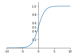
感受一下TensorFlow中的sigmoid函数:
import tensorflow as tf
x = tf.linspace(-5., 5.,6)
x
<tf.Tensor: id=3, shape=(6,), dtype=float32, numpy=array([-5., -3., -1., 1., 3., 5.], dtype=float32)>
有两种方式可以调用sigmoid函数:
tf.keras.activations.sigmoid(x)
<tf.Tensor: id=4, shape=(6,), dtype=float32, numpy=
array([0.00669285, 0.04742587, 0.26894143, 0.7310586 , 0.95257413,
0.9933072 ], dtype=float32)>
tf.sigmoid(x)
<tf.Tensor: id=5, shape=(6,), dtype=float32, numpy=
array([0.00669285, 0.04742587, 0.26894143, 0.7310586 , 0.95257413,
0.9933072 ], dtype=float32)>
看, 中所有值都映射到了[0,1]范围内。
sigmoid优缺点总结:
优点:输出的映射区间(0,1)内单调连续,非常适合用作输出层,并且比较容易求导。
缺点:具有软饱和性,即当输入x趋向于无穷的时候,它的导数会趋于0,导致很容易产生梯度消失。
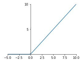
7.2.2 relu函数
Relu(Rectified Linear Units修正线性单元),是目前被使用最为频繁得激活函数,relu函数在x<0时,输出始终为0。由于x>0时,relu函数的导数为1,即保持输出为x,所以relu函数能够在x>0时保持梯度不断衰减,从而缓解梯度消失的问题,还能加快收敛速度,还能是神经网络具有稀疏性表达能力,这也是relu激活函数能够被使用在深层神经网络中的原因。由于当x<0时,relu函数的导数为0,导致对应的权重无法更新,这样的神经元被称为"神经元死亡"。
relu函数公式和图像如下:
在TensorFlow中,relu函数的参数情况比sigmoid复杂,我们先来看一下:
tf.keras.activations.relu( x, alpha=0.0, max_value=None, threshold=0 )
x:输入的变量
alpha:上图中左半边部分图像的斜率,也就是x值为负数(准确说应该是小于threshold)部分的斜率,默认为0
max_value:最大值,当x大于max_value时,输出值为max_value
threshold:起始点,也就是上面图中拐点处x轴的值
x = tf.linspace(-5., 5.,6)
x
<tf.Tensor: id=9, shape=(6,), dtype=float32, numpy=array([-5., -3., -1., 1., 3., 5.], dtype=float32)>
tf.keras.activations.relu(x)
<tf.Tensor: id=10, shape=(6,), dtype=float32, numpy=array([0., 0., 0., 1., 3., 5.], dtype=float32)>
tf.keras.activations.relu(x,alpha=2.)
<tf.Tensor: id=11, shape=(6,), dtype=float32, numpy=array([-10., -6., -2., 1., 3., 5.], dtype=float32)>
tf.keras.activations.relu(x,max_value=2.) # 大于2部分都将输出为2.
<tf.Tensor: id=16, shape=(6,), dtype=float32, numpy=array([0., 0., 0., 1., 2., 2.], dtype=float32)>
tf.keras.activations.relu(x,alpha=2., threshold=3.5) # 小于3.5的值按照alpha * (x - threshold)计算
<tf.Tensor: id=27, shape=(6,), dtype=float32, numpy=array([-17., -13., -9., -5., -1., 5.], dtype=float32)>
7.2.3 softmax函数
softmax函数是sigmoid函数的进化,在处理分类问题是很方便,它可以将所有输出映射到成概率的形式,即值在[0,1]范围且总和为1。例如输出变量为[1.5,4.4,2.0],经过softmax函数激活后,输出为[0.04802413, 0.87279755, 0.0791784 ],分别对应属于1、2、3类的概率。softmax函数数学公式如下:
tf.nn.softmax(tf.constant([[1.5,4.4,2.0]]))
<tf.Tensor: id=29, shape=(1, 3), dtype=float32, numpy=array([[0.04802413, 0.87279755, 0.0791784 ]], dtype=float32)>
tf.keras.activations.softmax(tf.constant([[1.5,4.4,2.0]]))
<tf.Tensor: id=31, shape=(1, 3), dtype=float32, numpy=array([[0.04802413, 0.87279755, 0.0791784 ]], dtype=float32)>
x = tf.random.uniform([1,5],minval=-2,maxval=2)
x
<tf.Tensor: id=38, shape=(1, 5), dtype=float32, numpy=
array([[ 1.9715171 , 0.49954653, -0.37836075, 1.6178164 , 0.80509186]],
dtype=float32)>
tf.keras.activations.softmax(x)
<tf.Tensor: id=39, shape=(1, 5), dtype=float32, numpy=
array([[0.42763966, 0.09813169, 0.04078862, 0.30023944, 0.13320053]],
dtype=float32)>
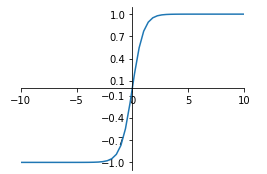
7.2.4 tanh函数
tanh函数无论是功能还是函数图像上斗鱼sigmoid函数十分相似,所以两者的优缺点也一样,区别在于tanh函数将值映射到[-1,1]范围,其数学公式和函数图像如下:
x = tf.linspace(-5., 5.,6)
x
<tf.Tensor: id=43, shape=(6,), dtype=float32, numpy=array([-5., -3., -1., 1., 3., 5.], dtype=float32)>
tf.keras.activations.tanh(x)
<tf.Tensor: id=44, shape=(6,), dtype=float32, numpy=
array([-0.99990916, -0.9950547 , -0.7615942 , 0.7615942 , 0.9950547 ,
0.99990916], dtype=float32)>
7.3 激活函数总结
神经网络中,隐藏层之间的输出大多需要通过激活函数来映射(当然,也可以不用,没有使用激活函数的层一般称为logits层),在构建模型是,需要根据实际数据情况选择激活函数。TensorFlow中的激活函数可不止这4个,本文只是介绍最常用的4个,当然,其他激活函数大多是这几个激活函数的变种。
TensorFlow2.0(8):误差计算——损失函数总结
8.1 均方差损失函数:MSE
均方误差(Mean Square Error),应该是最常用的误差计算方法了,数学公式为:
其中, 是真实值, 是预测值, 通常指的是batch_size,也有时候是指特征属性个数。
import tensorflow as tf
y = tf.random.uniform((5,),maxval=5,dtype=tf.int32) # 假设这是真实值
print(y)
y = tf.one_hot(y,depth=5) # 转为热独编码
print(y)
tf.Tensor([2 4 4 0 2], shape=(5,), dtype=int32)
tf.Tensor(
[[0. 0. 1. 0. 0.]
[0. 0. 0. 0. 1.]
[0. 0. 0. 0. 1.]
[1. 0. 0. 0. 0.]
[0. 0. 1. 0. 0.]], shape=(5, 5), dtype=float32)
y
<tf.Tensor: id=7, shape=(5, 5), dtype=float32, numpy=
array([[0., 0., 1., 0., 0.],
[0., 0., 0., 0., 1.],
[0., 0., 0., 0., 1.],
[1., 0., 0., 0., 0.],
[0., 0., 1., 0., 0.]], dtype=float32)>
pred = tf.random.uniform((5,),maxval=5,dtype=tf.int32) # 假设这是预测值
pred = tf.one_hot(pred,depth=5) # 转为热独编码
print(pred)
tf.Tensor(
[[0. 1. 0. 0. 0.]
[0. 0. 0. 1. 0.]
[1. 0. 0. 0. 0.]
[0. 0. 0. 1. 0.]
[0. 0. 0. 0. 1.]], shape=(5, 5), dtype=float32)
loss1 = tf.reduce_mean(tf.square(y-pred))
loss1
<tf.Tensor: id=19, shape=(), dtype=float32, numpy=0.4>
在tensorflow的losses模块中,提供能MSE方法用于求均方误差,注意简写MSE指的是一个方法,全写MeanSquaredError指的是一个类,通常通过方法的形式调用MSE使用这一功能。MSE方法返回的是每一对真实值和预测值之间的误差,若要求所有样本的误差需要进一步求平均值:
loss_mse_1 = tf.losses.MSE(y,pred)
loss_mse_1
<tf.Tensor: id=22, shape=(5,), dtype=float32, numpy=array([0.4, 0.4, 0.4, 0.4, 0.4], dtype=float32)>
loss_mse_2 = tf.reduce_mean(loss_mse_1)
loss_mse_2
<tf.Tensor: id=24, shape=(), dtype=float32, numpy=0.4>
一般而言,均方误差损失函数比较适用于回归问题中,对于分类问题,特别是目标输出为One-hot向量的分类任务中,下面要说的交叉熵损失函数就要合适的多。
8.2 交叉熵损失函数
交叉熵(Cross Entropy)是信息论中一个重要概念,主要用于度量两个概率分布间的差异性信息,交叉熵越小,两者之间差异越小,当交叉熵等于0时达到最佳状态,也即是预测值与真实值完全吻合。先给出交叉熵计算公式:
其中, 是真实分布的概率, 是模型通过数据计算出来的概率估计。
不理解?没关系,我们通过一个例子来说明。假设对于一个分类问题,其可能结果有5类,由 表示,有一个样本 ,其真实结果是属于第2类,用One-hot编码表示就是 ,也就是上面公司中的 。现在有两个模型,对样本 的预测结果分别是 和 ,也就是上面公式中的 。从直觉上判断,我们会认为第一个模型预测要准确一些,因为它更加肯定 属于第二类,不过,我们需要通过科学的量化分析对比来证明这一点:
第一个模型交叉熵:
第二个模型交叉熵:
可见, ,所以第一个模型的结果更加可靠。
在TensorFlow中,计算交叉熵通过tf.losses模块中的categorical_crossentropy()方法。
tf.losses.categorical_crossentropy([0,1,0,0,0],[0.1, 0.7, 0.05, 0.05, 0.1])
<tf.Tensor: id=41, shape=(), dtype=float32, numpy=0.35667497>
tf.losses.categorical_crossentropy([0,1,0,0,0],[0, 0.6, 0.2, 0.1, 0.1])
<tf.Tensor: id=58, shape=(), dtype=float32, numpy=0.5108256>
模型在最后一层隐含层的输出可能并不是概率的形式,不过可以通过softmax函数转换为概率形式输出,然后计算交叉熵,但有时候可能会出现不稳定的情况,即输出结果是NAN或者inf,这种情况下可以通过直接计算隐藏层输出结果的交叉熵,不过要给categorical_crossentropy()方法传递一个from_logits=True参数。
x = tf.random.normal([1,784])
w = tf.random.normal([784,2])
b = tf.zeros([2])
logits = x@w + b # 最后一层没有激活函数的层称为logits层
logits
<tf.Tensor: id=75, shape=(1, 2), dtype=float32, numpy=array([[ 5.236802, 18.843138]], dtype=float32)>
prob = tf.math.softmax(logits, axis=1) # 转换为概率的形式
prob
<tf.Tensor: id=77, shape=(1, 2), dtype=float32, numpy=array([[1.2326591e-06, 9.9999881e-01]], dtype=float32)>
tf.losses.categorical_crossentropy([0,1],logits,from_logits=True) # 通过logits层直接计算交叉熵
<tf.Tensor: id=112, shape=(1,), dtype=float32, numpy=array([1.1920922e-06], dtype=float32)>
tf.losses.categorical_crossentropy([0,1],prob) # 通过转换后的概率计算交叉熵
<tf.Tensor: id=128, shape=(1,), dtype=float32, numpy=array([1.1920936e-06], dtype=float32)>
TensorFlow2.0(9):神器级可视化工具TensorBoard
9.1神器级的TensorBoard
TensorBoard是TensorFlow中的又一神器级工具,想用户提供了模型可视化的功能。我们都知道,在构建神经网络模型时,只要模型开始训练,很多细节对外界来说都是不可见的,参数如何变化,准确率怎么样了,loss还在减小吗,这些问题都很难弄明白。但是,TensorBoard通过结合web应用为我们提供了这一功能,它将模型训练过程的细节以图表的形式通过浏览器可视化得展现在我们眼前,通过这种方式我们可以清晰感知weight、bias、accuracy的变化,把握训练的趋势。
本文介绍两种使用TensorBoard的方式。不过,无论使用那种方式,请先启动TensorBoard的web应用,这个web应用读取模型训练时的日志数据,每隔30秒更新到网页端。在TensorFlow2.0中,TensorBoard是默认安装好的,所以,可以直接根据以下命令启动:
tensorboard --logdir "/home/chb/jupyter/logs"
logdir指的是日志目录,每次训练模型时,TensorBoard会在日志目录中创建一个子目录,在其中写入日志,TensorBoard的web应用正是通过日志来感知模型的训练状态,然后更新到网页端。
如果命令成功运行,可以通过本地的6006端口打开网页,但是,此时打开的页面时下面这个样子,因为还没有开始训练模型,更没有将日志写入到指定的目录。
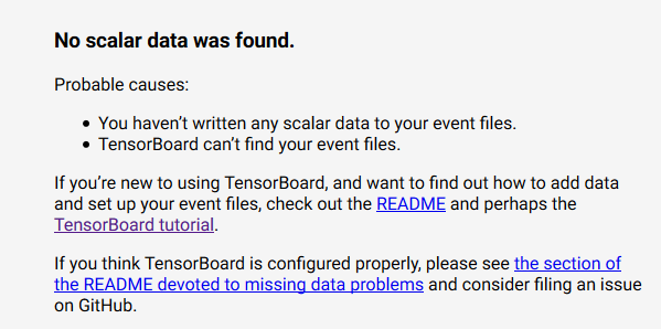
要将训练数据写入指定目录就必须将TensorBoard嵌入模型的训练过程,TensorFlow介绍了两种方式。下面,我们通过mnist数据集训练过程来介绍着两种方式。
9.2 在Model.fit()中使用TensorBoard
import tensorflow as tf
import tensorboard
import datetime
mnist = tf.keras.datasets.mnist
(x_train, y_train),(x_test, y_test) = mnist.load_data()
x_train, x_test = x_train / 255.0, x_test / 255.0
def create_model():
return tf.keras.models.Sequential([
tf.keras.layers.Flatten(input_shape=(28, 28)),
tf.keras.layers.Dense(512, activation='relu'),
tf.keras.layers.Dropout(0.2),
tf.keras.layers.Dense(10, activation='softmax')
])
model = create_model()
model.compile(optimizer='adam', loss='sparse_categorical_crossentropy', metrics=['accuracy'])
# 定义日志目录,必须是启动web应用时指定目录的子目录,建议使用日期时间作为子目录名
log_dir="/home/chb/jupyter/logs/" + datetime.datetime.now().strftime("%Y%m%d-%H%M%S")
tensorboard_callback = tf.keras.callbacks.TensorBoard(log_dir=log_dir, histogram_freq=1) # 定义TensorBoard对象
model.fit(x=x_train,
y=y_train,
epochs=5,
validation_data=(x_test, y_test),
callbacks=[tensorboard_callback]) # 将定义好的TensorBoard对象作为回调传给fit方法,这样就将TensorBoard嵌入了模型训练过程
Train on 60000 samples, validate on 10000 samples
Epoch 1/5
60000/60000 [==============================] - 4s 71us/sample - loss: 0.2186 - accuracy: 0.9349 - val_loss: 0.1180 - val_accuracy: 0.9640
Epoch 2/5
60000/60000 [==============================] - 4s 66us/sample - loss: 0.0972 - accuracy: 0.9706 - val_loss: 0.0754 - val_accuracy: 0.9764
Epoch 3/5
60000/60000 [==============================] - 4s 66us/sample - loss: 0.0685 - accuracy: 0.9781 - val_loss: 0.0696 - val_accuracy: 0.9781
Epoch 4/5
60000/60000 [==============================] - 4s 66us/sample - loss: 0.0527 - accuracy: 0.9831 - val_loss: 0.0608 - val_accuracy: 0.9808
Epoch 5/5
60000/60000 [==============================] - 4s 66us/sample - loss: 0.0444 - accuracy: 0.9859 - val_loss: 0.0637 - val_accuracy: 0.9803
<tensorflow.python.keras.callbacks.History at 0x7f9b690893d0>
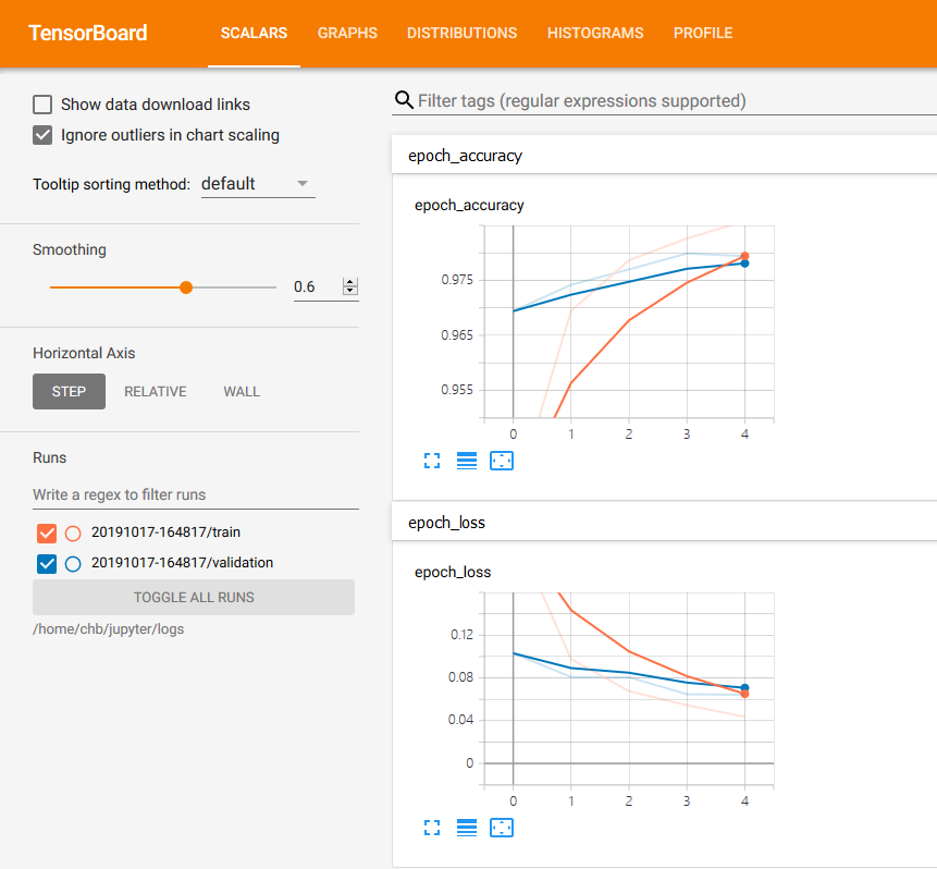
通过TensorBoard提供的图标,我们可以清楚的知道训练模型时loss和accuracy在每一个epoch中是怎么变化的,甚至,在网页菜单栏我们可以看到,TensorBoard提供了查看其他内容的功能:
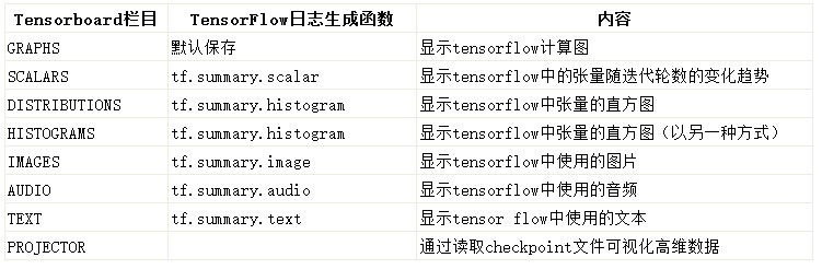
在 scalars 下可以看到 accuracy,cross entropy,dropout,bias,weights 等的趋势。
在 images 和 audio 下可以看到输入的数据。
在 graphs 中可以看到模型的结构。
在 histogram 可以看到 activations,gradients 或者 weights 等变量的每一步的分布,越靠前面就是越新的步数的结果。
distribution 和 histogram 是两种不同的形式,可以看到整体的状况。
在 embedding 中可以看到用 PCA 主成分分析方法将高维数据投影到 3D 空间后的数据的关系。
这就是TensorBoard提供的功能,不可为不强大。这里,我们在介绍一下TensorBoard构造方法中的参数:工具在Tensorflow中是非常常用的其参数解释如下:
log_dir:保存TensorBoard要解析的日志文件的目录的路径。
histogram_freq:频率(在epoch中),计算模型层的激活和权重直方图。如果设置为0,则不会计算直方图。必须为直方图可视化指定验证数据(或拆分)。
write_graph:是否在TensorBoard中可视化图像。当write_graph设置为True时,日志文件可能会变得非常大。
write_grads:是否在TensorBoard中可视化渐变直方图。histogram_freq必须大于0。
batch_size:用以直方图计算的传入神经元网络输入批的大小。
write_images:是否在TensorBoard中编写模型权重以显示为图像。
embeddings_freq:将保存所选嵌入层的频率(在epoch中)。如果设置为0,则不会计算嵌入。要在TensorBoard的嵌入选项卡中显示的数据必须作为embeddings_data传递。
embeddings_layer_names:要关注的层名称列表。如果为None或空列表,则将监测所有嵌入层。
embeddings_metadata:将层名称映射到文件名的字典,其中保存了此嵌入层的元数据。如果相同的元数据文件用于所有嵌入层,则可以传递字符串。
embeddings_data:要嵌入在embeddings_layer_names指定的层的数据。Numpy数组(如果模型有单个输入)或Numpy数组列表(如果模型有多个输入)。
update_freq:‘batch’或’epoch’或整数。使用’batch’时,在每个batch后将损失和指标写入TensorBoard。这同样适用’epoch’。如果使用整数,比方说1000,回调将会在每1000个样本后将指标和损失写入TensorBoard。请注意,过于频繁地写入TensorBoard会降低您的训练速度。还有可能引发的异常:
ValueError:如果设置了histogram_freq且未提供验证数据。
9.3 在其他功能函数中嵌入TensorBoard
在训练模型时,我们可以在 tf.GradientTape()等等功能函数中个性化得通过tf.summary()方法指定需要TensorBoard展示的参数。
同样适用fashion_mnist数据集建立一个模型:
import datetime
import tensorflow as tf
from tensorflow import keras
from tensorflow.keras import datasets, layers, optimizers, Sequential ,metrics
def preprocess(x, y):
x = tf.cast(x, dtype=tf.float32) / 255.
y = tf.cast(y, dtype=tf.int32)
return x, y
(x, y), (x_test, y_test) = datasets.fashion_mnist.load_data()
db = tf.data.Dataset.from_tensor_slices((x, y))
db = db.map(preprocess).shuffle(10000).batch(128)
db_test = tf.data.Dataset.from_tensor_slices((x_test, y_test))
db_test = db_test.map(preprocess).batch(128)
model = Sequential([
layers.Dense(256, activation=tf.nn.relu), # [b, 784] --> [b, 256]
layers.Dense(128, activation=tf.nn.relu), # [b, 256] --> [b, 128]
layers.Dense(64, activation=tf.nn.relu), # [b, 128] --> [b, 64]
layers.Dense(32, activation=tf.nn.relu), # [b, 64] --> [b, 32]
layers.Dense(10) # [b, 32] --> [b, 10]
]
)
model.build(input_shape=[None,28*28])
model.summary()
optimizer = optimizers.Adam(lr=1e-3)#1e-3
# 指定日志目录
log_dir="/home/chb/jupyter/logs/" + datetime.datetime.now().strftime("%Y%m%d-%H%M%S")
summary_writer = tf.summary.create_file_writer(log_dir) # 创建日志文件句柄
Model: "sequential_3"
_________________________________________________________________
Layer (type) Output Shape Param #
=================================================================
dense_15 (Dense) multiple 200960
_________________________________________________________________
dense_16 (Dense) multiple 32896
_________________________________________________________________
dense_17 (Dense) multiple 8256
_________________________________________________________________
dense_18 (Dense) multiple 2080
_________________________________________________________________
dense_19 (Dense) multiple 330
=================================================================
Total params: 244,522
Trainable params: 244,522
Non-trainable params: 0
_________________________________________________________________
db_iter = iter(db)
images = next(db_iter)
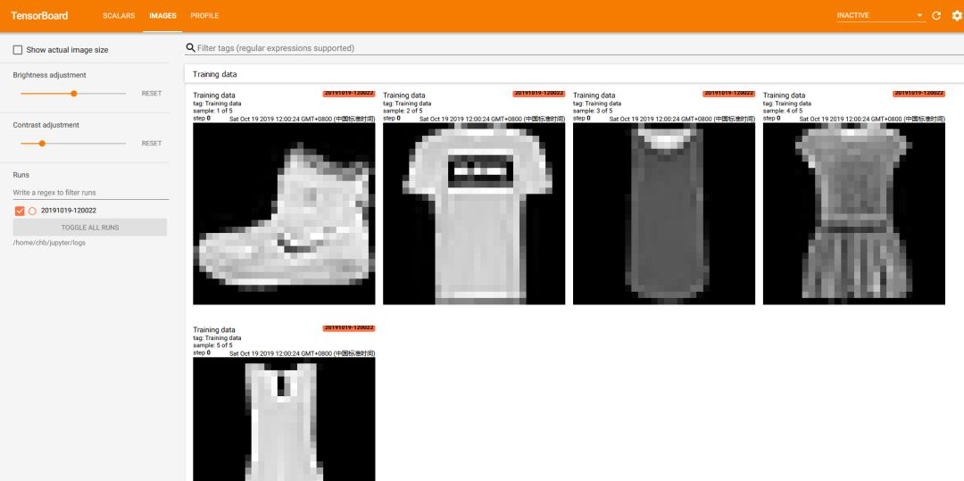
# 必须进行reshape,第一个纬度是图片数量或者说簇大小,28*28是图片大小,1是chanel,因为只灰度图片所以是1
images = tf.reshape(x, (-1, 28, 28, 1))
with summary_writer.as_default(): # 将第一个簇的图片写入TensorBoard
tf.summary.image('Training data', images, max_outputs=5, step=0) # max_outputs设置最大显示图片数量
tf.summary.trace_on(graph=True, profiler=True)
for epoch in range(30):
train_loss = 0
train_num = 0
for step, (x, y) in enumerate(db):
x = tf.reshape(x, [-1, 28*28])
with tf.GradientTape() as tape:
logits = model(x)
y_onehot = tf.one_hot(y,depth=10)
loss_mse = tf.reduce_mean(tf.losses.MSE(y_onehot, logits))
loss_ce = tf.losses.categorical_crossentropy(y_onehot, logits, from_logits=True)
loss_ce = tf.reduce_mean(loss_ce) # 计算整个簇的平均loss
grads = tape.gradient(loss_ce, model.trainable_variables) # 计算梯度
optimizer.apply_gradients(zip(grads, model.trainable_variables)) # 更新梯度
train_loss += float(loss_ce)
train_num += x.shape[0]
loss = train_loss / train_num # 计算每一次迭代的平均loss
with summary_writer.as_default(): # 将loss写入TensorBoard
tf.summary.scalar('train_loss', train_loss, step=epoch)
total_correct = 0
total_num = 0
for x,y in db_test: # 用测试集验证每一次迭代后的准确率
x = tf.reshape(x, [-1, 28*28])
logits = model(x)
prob = tf.nn.softmax(logits, axis=1)
pred = tf.argmax(prob, axis=1)
pred = tf.cast(pred, dtype=tf.int32)
correct = tf.equal(pred, y)
correct = tf.reduce_sum(tf.cast(correct, dtype=tf.int32))
total_correct += int(correct)
total_num += x.shape[0]
acc = total_correct / total_num # 平均准确率
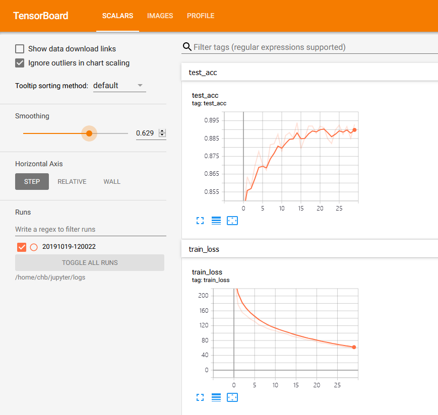
with summary_writer.as_default(): # 将acc写入TensorBoard
tf.summary.scalar('test_acc', acc, step=epoch)
print(epoch, 'train_loss:',loss,'test_acc:', acc)
0 train_loss: 0.004282377735277017 test_acc: 0.8435
1 train_loss: 0.0029437638364732265 test_acc: 0.8635
2 train_loss: 0.0025979293311635654 test_acc: 0.858
3 train_loss: 0.0024499946276346843 test_acc: 0.8698
4 train_loss: 0.0022926158788303536 test_acc: 0.8777
5 train_loss: 0.002190616005907456 test_acc: 0.8703
6 train_loss: 0.0020421392366290095 test_acc: 0.8672
7 train_loss: 0.001972314653545618 test_acc: 0.8815
8 train_loss: 0.0018821696805457274 test_acc: 0.882
9 train_loss: 0.0018143038821717104 test_acc: 0.8874
10 train_loss: 0.0017742110469688972 test_acc: 0.8776
11 train_loss: 0.0017088291154553493 test_acc: 0.8867
12 train_loss: 0.0016564140267670154 test_acc: 0.8883
13 train_loss: 0.001609446036318938 test_acc: 0.8853
14 train_loss: 0.0015313156222303709 test_acc: 0.8939
15 train_loss: 0.0014887714397162199 test_acc: 0.8793
16 train_loss: 0.001450310030952096 test_acc: 0.8853
17 train_loss: 0.001389076333368818 test_acc: 0.892
18 train_loss: 0.0013547154798482855 test_acc: 0.892
19 train_loss: 0.0013331565233568351 test_acc: 0.8879
20 train_loss: 0.001276270254018406 test_acc: 0.8919
21 train_loss: 0.001228199392867585 test_acc: 0.8911
22 train_loss: 0.0012089030482495824 test_acc: 0.8848
23 train_loss: 0.0011713500657429298 test_acc: 0.8822
24 train_loss: 0.0011197352315609655 test_acc: 0.8898
25 train_loss: 0.0011078068762707214 test_acc: 0.8925
26 train_loss: 0.0010750674727062384 test_acc: 0.8874
27 train_loss: 0.0010422117731223503 test_acc: 0.8917
28 train_loss: 0.0010244071063275138 test_acc: 0.8851
29 train_loss: 0.0009715937084207933 test_acc: 0.8929
TensorBoard中web界面如下:
TensorFlow2.0(10):加载自定义图片数据集到Dataset
前面的博客中我们说过,在加载数据和预处理数据时使用tf.data.Dataset对象将极大将我们从建模前的数据清理工作中释放出来,那么,怎么将自定义的数据集加载为DataSet对象呢?这对很多新手来说都是一个难题,因为绝大多数案例教学都是以mnist数据集作为例子讲述如何将数据加载到Dataset中,而英文资料对这方面的介绍隐藏得有点深。本文就来捋一捋如何加载自定义的图片数据集实现图片分类,后续将继续介绍如何加载自定义的text、mongodb等数据。
10.1加载自定义图片数据集
如果你已有数据集,那么,请将所有数据存放在同一目录下,然后将不同类别的图片分门别类地存放在不同的子目录下,目录树如下所示:
$ tree flower_photos -L 1
flower_photos
├── daisy
├── dandelion
├── LICENSE.txt
├── roses
├── sunflowers
└── tulips
所有的数据都存放在flower_photos目录下,每一个子目录(daisy、dandelion等等)存放的都是一个类别的图片。如果你已有自己的数据集,那就按上面的结构来存放,如果没有,想操作学习一下,你可以通过下面代码下载上述图片数据集:
import tensorflow as tf
import pathlib
data_root_orig = tf.keras.utils.get_file(origin='https://storage.googleapis.com/download.tensorflow.org/example_images/flower_photos.tgz',
fname='flower_photos', untar=True)
data_root = pathlib.Path(data_root_orig)
print(data_root) # 打印出数据集所在目录
下载好后,建议将整个flower_photos目录移动到项目根目录下。
import tensorflow as tf
import random
import pathlib
data_path = pathlib.Path('./data/flower_photos')
all_image_paths = list(data_path.glob('*/*'))
all_image_paths = [str(path) for path in all_image_paths] # 所有图片路径的列表
random.shuffle(all_image_paths) # 打散
image_count = len(all_image_paths)
image_count
3670
查看一下前5张:
all_image_paths[:5]
['data/flower_photos/sunflowers/9448615838_04078d09bf_n.jpg',
'data/flower_photos/roses/15222804561_0fde5eb4ae_n.jpg',
'data/flower_photos/daisy/18622672908_eab6dc9140_n.jpg',
'data/flower_photos/roses/459042023_6273adc312_n.jpg',
'data/flower_photos/roses/16149016979_23ef42b642_m.jpg']
读取图片的同时,我们也不能忘记图片与标签的对应,要创建一个对应的列表来存放图片标签,不过,这里所说的标签不是daisy、dandelion这些具体分类名,而是整型的索引,毕竟在建模的时候y值一般都是整型数据,所以要创建一个字典来建立分类名与标签的对应关系:
label_names = sorted(item.name for item in data_path.glob('*/') if item.is_dir())
label_names
['daisy', 'dandelion', 'roses', 'sunflowers', 'tulips']
label_to_index = dict((name, index) for index, name in enumerate(label_names))
label_to_index
{'daisy': 0, 'dandelion': 1, 'roses': 2, 'sunflowers': 3, 'tulips': 4}
all_image_labels = [label_to_index[pathlib.Path(path).parent.name] for path in all_image_paths]
for image, label in zip(all_image_paths[:5], all_image_labels[:5]):
print(image, ' ---> ', label)
data/flower_photos/sunflowers/9448615838_04078d09bf_n.jpg ---> 3
data/flower_photos/roses/15222804561_0fde5eb4ae_n.jpg ---> 2
data/flower_photos/daisy/18622672908_eab6dc9140_n.jpg ---> 0
data/flower_photos/roses/459042023_6273adc312_n.jpg ---> 2
data/flower_photos/roses/16149016979_23ef42b642_m.jpg ---> 2
好了,现在我们可以创建一个Dataset了:
ds = tf.data.Dataset.from_tensor_slices((all_image_paths, all_image_labels))
不过,这个ds可不是我们想要的,毕竟,里面的元素只是图片路径,所以我们要进一步处理。这个处理包含读取图片、重新设置图片大小、归一化、转换类型等操作,我们将这些操作统统定义到一个方法里:
def load_and_preprocess_from_path_label(path, label):
image = tf.io.read_file(path) # 读取图片
image = tf.image.decode_jpeg(image, channels=3)
image = tf.image.resize(image, [192, 192]) # 原始图片大小为(266, 320, 3),重设为(192, 192)
image /= 255.0 # 归一化到[0,1]范围
return image, label
image_label_ds = ds.map(load_and_preprocess_from_path_label)
image_label_ds
<MapDataset shapes: ((192, 192, 3), ()), types: (tf.float32, tf.int32)>
这时候,其实就已经将自定义的图片数据集加载到了Dataset对象中,不过,我们还能秀,可以继续shuffle随机打散、分割成batch、数据repeat操作。这些操作有几点需要注意:
(1)先shuffle、repeat、batch三种操作顺序有讲究:
在repeat之后shuffle,会在epoch之间数据随机(当有些数据出现两次的时候,其他数据还没有出现过)
在batch之后shuffle,会打乱batch的顺序,但是不会在batch之间打乱数据。
(2)shuffle操作时,buffer_size越大,打乱效果越好,但消耗内存越大,可能造成延迟。
推荐通过使用 tf.data.Dataset.apply 方法和融合过的 tf.data.experimental.shuffle_and_repeat 函数来执行这些操作:
ds = image_label_ds.apply(tf.data.experimental.shuffle_and_repeat(buffer_size=image_count))
BATCH_SIZE = 32
ds = ds.batch(BATCH_SIZE)
好了,至此,本文内容其实就结束了,因为已经将自定义的图片数据集加载到了Dataset中。
10.2扩展阅读
上面的方法是简单的在每次epoch迭代中单独读取每个文件,在本地使用 CPU 训练时这个方法是可行的,但是可能不足以进行GPU训练并且完全不适合任何形式的分布式训练。
可以使用tf.data.Dataset.cache在epoch迭代过程间缓存计算结果。这能极大提升程序效率,特别是当内存能容纳全部数据时。
在被预处理之后(解码和调整大小),图片就被缓存了:
ds = image_label_ds.cache() # 缓存
ds = ds.apply(tf.data.experimental.shuffle_and_repeat(buffer_size=image_count))
使用内存缓存的一个缺点是必须在每次运行时重建缓存,这使得每次启动数据集时有相同的启动延迟。如果内存不够容纳数据,使用一个缓存文件:
ds = image_label_ds.cache(filename='./cache.tf-data')
ds = ds.apply(tf.data.experimental.shuffle_and_repeat(buffer_size=image_count))
TensorFlow2.0(11):tf.keras建模三部曲
Keras是一个基于Python编写的高层神经网络API,凭借用户友好性、模块化以及易扩展等有点大受好评,考虑到Keras的优良特性以及它的受欢迎程度,TensorFlow2.0中将Keras的代码吸收了进来,化身为tf.keras模块供用户使用。
使用tf.keras提供的高层API,可以轻松得完成建模三部曲——模型构建、训练、评估等工作。下面我们分别来说说如何使用tf.keras完成这三部曲。
11.1 模型构建
我们知道,神经网络模型就是层的堆叠,tf.keras提供的Sequential类对象就是层容器,可以轻松实现对层的堆叠,创建网络模型。用Sequential创建一个全连接网络模型:
import tensorflow as tf
from tensorflow import keras # 为方便使用,keras一般单独导入
from tensorflow.keras import layers
model = tf.keras.Sequential()
# 往模型中添加一个有64个神经元组成的层,激活函数为relu:
model.add(layers.Dense(64, activation='relu'))
# 再添加一个:
model.add(layers.Dense(64, activation='relu'))
# 添加一个有10个神经元的softmax层作为输出层:
model.add(layers.Dense(10, activation='softmax'))
也可以在使用Sequential实例化模型时,通过传入由层组成的列表来添加层。我们换一种方式实现上面的模型构建过程,两种方式是完全等效的:
model = tf.keras.Sequential([
layers.Dense(64, activation='relu'),
layers.Dense(64, activation='relu'),
layers.Dense(10, activation='softmax')]
)
你看,用tf.keras创建一个模型,就是这么简单,只需要往Sequential中传入一个个tf.keras.layers定义的层就好了。进一步的,我们研究一下tf.keras.layers怎么个性化地创建层。
定义神经网络层通过tf.keras.layers模块中的Dense类实现,Dense类构造参数如下:
units:指定神经元个数,必须是一个正整数。
activation:激活函数,可以是可以是一个可调用对象或标识一个对象的字符串
use_bias:布尔型,是否使用是否使用偏置项
kernel_initializer和bias_initializer:权值、偏置初始化方法,可以是一个可调用对象或标识一个对象的字符串
kernel_regularizer和bias_regularizer:对权值、偏置进行正则化的方法,可以是一个可调用对象或标识一个对象的字符串
activity_regularizer:对层的输出进行正则化的方法,可以是一个可调用对象或标识一个对象的字符串
kernel_constraint和bias_constraint:对权值矩阵、偏置矩阵的约束方法,可以是一个可调用对象或标识一个对象的字符串
# 有64个神经元,激活函数为sigmoid的层
layers.Dense(64, activation='sigmoid')
# 或者:
layers.Dense(64, activation=tf.keras.activations.sigmoid)
# 对权值矩阵进行正则化:
layers.Dense(64, kernel_regularizer=tf.keras.regularizers.l1(0.01))
# 对偏置向量进行正则化:
layers.Dense(64, bias_regularizer=tf.keras.regularizers.l2(0.01))
# 指定权值随机正交初始化:
layers.Dense(64, kernel_initializer='orthogonal')
# 指定偏置为常数:
layers.Dense(64, bias_initializer=tf.keras.initializers.Constant(2.0))
<tensorflow.python.keras.layers.core.Dense at 0x7f486247abd0>
11.2 训练模型
配置:compile()
建立好模型之后,接下来当然是要进行训练模型了。不过,在训练前还需要做一些配置工作,例如指定优化器、损失函数、评估指标等,这些配置参数的过程一般通过tf.keras.Model.compile方法进行,先来熟悉一下tf.keras.Model.compile方法的三个常用参数:
optimizer:tf.keras.optimizers模块中的优化器实例化对象,例如 tf.keras.optimizers.Adam或 tf.keras.optimizers.SGD的实例化对象,当然也可以使用字符串来指代优化器,例如'adam'和'sgd'。
loss:损失函数,例如交叉熵、均方差等,通常是tf.keras.losses模块中定义的可调用对象,也可以用用于指代损失函数的字符串。
metrics:元素为评估方法的list,通常是定义在tf.keras.metrics模块中定义的可调用对象,也可以用于指代评估方法的字符串。
在知道怎么配置模型训练参数后,就可以根据实际应用情况合理选择优化器、损失函数、评估方法等:
# 回归模型
model.compile(optimizer=tf.keras.optimizers.Adam(0.01), # 指定优化器,学习率为0.01
loss='mse', # 指定均方差作为损失函数
metrics=['mae']) # 添加绝对值误差作为评估方法
# 分类模型
model.compile(optimizer=tf.keras.optimizers.RMSprop(0.01),
loss=tf.keras.losses.CategoricalCrossentropy(), # 分类模型多用交叉熵作为损失函数
metrics=[tf.keras.metrics.CategoricalAccuracy()])
通过compile()配置好模型后,就可以开始训练了。tf.keras中提供了fit()方法对模型进行训练,先来看看fit()方法的主要参数:
x和y:训练数据和目标数据
epochs:训练周期数,每一个周期都是对训练数据集的一次完整迭代
batch_size:簇的大小,一般在数据集是numpy数组类型时使用
validation_data:验证数据集,模型训练时,如果你想通过一个额外的验证数据集来监测模型的性能变换,就可以通过这个参数传入验证数据集
verbose:日志显示方式,verbose=0为不在标准输出流输出日志信息,verbose=1为输出进度条记录,verbose=2为每个epoch输出一行记录
callbacks:回调方法组成的列表,一般是定义在tf.keras.callbacks中的方法
validation_split:从训练数据集抽取部分数据作为验证数据集的比例,是一个0到1之间的浮点数。这一参数在输入数据为dataset对象、生成器、keras.utils.Sequence对象是无效。
shuffle:是否在每一个周期开始前打乱数据
下面分别说说如何使用fit()方法结合numpy数据和tf.data.Dataset数据进行模型训练。
import numpy as np
data = np.random.random((1000, 32))
labels = np.random.random((1000, 10))
model.fit(data, labels, epochs=10, batch_size=32)
Train on 1000 samples
Epoch 1/10
1000/1000 [==============================] - 1s 554us/sample - loss: 206.2688 - categorical_accuracy: 0.1050
Epoch 2/10
1000/1000 [==============================] - 0s 34us/sample - loss: 911.8347 - categorical_accuracy: 0.0990
Epoch 3/10
1000/1000 [==============================] - 0s 30us/sample - loss: 1879.7505 - categorical_accuracy: 0.0980
Epoch 4/10
1000/1000 [==============================] - 0s 28us/sample - loss: 3141.3959 - categorical_accuracy: 0.0940
Epoch 5/10
1000/1000 [==============================] - 0s 36us/sample - loss: 4673.7791 - categorical_accuracy: 0.1010
Epoch 6/10
1000/1000 [==============================] - 0s 36us/sample - loss: 6526.8757 - categorical_accuracy: 0.0960
Epoch 7/10
1000/1000 [==============================] - 0s 31us/sample - loss: 8571.8533 - categorical_accuracy: 0.1020
Epoch 8/10
1000/1000 [==============================] - 0s 33us/sample - loss: 11070.1039 - categorical_accuracy: 0.0970
Epoch 9/10
1000/1000 [==============================] - 0s 36us/sample - loss: 13533.4661 - categorical_accuracy: 0.1050
Epoch 10/10
1000/1000 [==============================] - 0s 25us/sample - loss: 17259.2291 - categorical_accuracy: 0.1000
<tensorflow.python.keras.callbacks.History at 0x7f74a4755650>
如何使用验证数据集的话,可以这样:
import numpy as np
data = np.random.random((1000, 32))
labels = np.random.random((1000, 10))
val_data = np.random.random((100, 32))
val_labels = np.random.random((100, 10))
model.fit(data, labels, epochs=10, batch_size=32,
validation_data=(val_data, val_labels)) # 验证数据集以元组的形式传入
Train on 1000 samples, validate on 100 samples
Epoch 1/10
1000/1000 [==============================] - 0s 34us/sample - loss: 67219.8359 - categorical_accuracy: 0.0960 - val_loss: 55306.6777 - val_categorical_accuracy: 0.1000
Epoch 2/10
1000/1000 [==============================] - 0s 32us/sample - loss: 73732.5724 - categorical_accuracy: 0.0920 - val_loss: 89920.2088 - val_categorical_accuracy: 0.1100
Epoch 3/10
1000/1000 [==============================] - 0s 50us/sample - loss: 79956.1480 - categorical_accuracy: 0.1020 - val_loss: 101092.6750 - val_categorical_accuracy: 0.1000
Epoch 4/10
1000/1000 [==============================] - 0s 36us/sample - loss: 84322.9844 - categorical_accuracy: 0.0970 - val_loss: 117610.5700 - val_categorical_accuracy: 0.1000
Epoch 5/10
1000/1000 [==============================] - 0s 38us/sample - loss: 91992.0751 - categorical_accuracy: 0.1130 - val_loss: 94200.0838 - val_categorical_accuracy: 0.1000
Epoch 6/10
1000/1000 [==============================] - 0s 38us/sample - loss: 97189.2044 - categorical_accuracy: 0.0910 - val_loss: 89020.5294 - val_categorical_accuracy: 0.1100
Epoch 7/10
1000/1000 [==============================] - 0s 33us/sample - loss: 107109.9905 - categorical_accuracy: 0.0930 - val_loss: 102350.4259 - val_categorical_accuracy: 0.1200
Epoch 8/10
1000/1000 [==============================] - 0s 41us/sample - loss: 114450.2496 - categorical_accuracy: 0.1010 - val_loss: 102719.3653 - val_categorical_accuracy: 0.1100
Epoch 9/10
1000/1000 [==============================] - 0s 41us/sample - loss: 124694.8415 - categorical_accuracy: 0.0950 - val_loss: 142269.8362 - val_categorical_accuracy: 0.1100
Epoch 10/10
1000/1000 [==============================] - 0s 44us/sample - loss: 131952.7791 - categorical_accuracy: 0.0800 - val_loss: 158925.8294 - val_categorical_accuracy: 0.0900
<tensorflow.python.keras.callbacks.History at 0x7f749c548810>
11.3 评估与预测
是骡子是马,拉出来溜溜就知道了,训练好的模型性能如何,评估测试一下就知道了。可以使用模型自带的evaluate()方法和predict()方法对模型进行评估和预测。
# 如果是numpy数据,可以这么使用
data = np.random.random((1000, 32))
labels = np.random.random((1000, 10))
model.evaluate(data, labels, batch_size=32)
0s 17us/sample - loss: 161163.7180 - categorical_accuracy: 0.0930
[153591.27975, 0.093]
# 如果数Dataset对象,可以这么使用
dataset = tf.data.Dataset.from_tensor_slices((data, labels))
dataset = dataset.batch(32)
model.evaluate(dataset)
32/32 [==============================] - 0s 579us/step - loss: 153946.2378 - categorical_accuracy: 0.0930
[153946.23779296875, 0.093]
使用predict()方法进行预测:
# numpy数据
result = model.predict(data, batch_size=32)
print(result.shape)
(1000, 10)
# dataset数据
result = model.predict(dataset)
print(result.shape)
(1000, 10)
TensorFlow2.0(12):模型保存与序列化
模型训练好之后,我们就要想办法将其持久化保存下来,不然关机或者程序退出后模型就不复存在了。本文介绍两种持久化保存模型的方法:
在介绍这两种方法之前,我们得先创建并训练好一个模型,还是以mnist手写数字识别数据集训练模型为例:
import tensorflow as tf
from tensorflow import keras
from tensorflow.keras import layers, optimizers, Sequential
model = Sequential([ # 创建模型
layers.Dense(256, activation=tf.nn.relu),
layers.Dense(128, activation=tf.nn.relu),
layers.Dense(64, activation=tf.nn.relu),
layers.Dense(32, activation=tf.nn.relu),
layers.Dense(10)
]
)
(x_train, y_train), (x_test, y_test) = keras.datasets.mnist.load_data()
x_train = x_train.reshape(60000, 784).astype('float32') / 255
x_test = x_test.reshape(10000, 784).astype('float32') / 255
model.compile(loss='sparse_categorical_crossentropy',
optimizer=keras.optimizers.RMSprop())
history = model.fit(x_train, y_train, # 进行简单的1次迭代训练
batch_size=64,
epochs=1)
Train on 60000 samples
60000/60000 [==============================] - 3s 46us/sample - loss: 2.3700
方法一:model.save()
通过模型自带的save()方法可以将模型保存到一个指定文件中,保存的内容包括:
模型的结构
模型的权重参数
通过compile()方法配置的模型训练参数
优化器及其状态
model.save('mymodels/mnist.h5')
使用save()方法保存后,在mymodels目录下就会有一个mnist.h5文件。需要使用模型时,通过keras.models.load_model()方法从文件中再次加载即可。
new_model = keras.models.load_model('mymodels/mnist.h5')
WARNING:tensorflow:Sequential models without an `input_shape` passed to the first layer cannot reload their optimizer state. As a result, your model isstarting with a freshly initialized optimizer.
新加载出来的new_model在结构、功能、参数各方面与model是一样的。
通过save()方法,也可以将模型保存为SavedModel 格式。SavedModel格式是TensorFlow所特有的一种序列化文件格式,其他编程语言实现的TensorFlow中同样支持:
model.save('mymodels/mnist_model', save_format='tf') # 将模型保存为SaveModel格式
WARNING:tensorflow:From /home/chb/anaconda3/envs/study_python/lib/python3.7/site-packages/tensorflow_core/python/ops/resource_variable_ops.py:1781: calling BaseResourceVariable.__init__ (from tensorflow.python.ops.resource_variable_ops) with constraint is deprecated and will be removed in a future version.
Instructions for updating:
If using Keras pass *_constraint arguments to layers.
INFO:tensorflow:Assets written to: mymodels/mnist_model/assets
new_model = keras.models.load_model('mymodels/mnist_model') # 加载模型
print(keras.models.__dir__())
['__name__', '__doc__', '__package__', '__loader__', '__spec__', '__path__', '__file__', '__cached__', '__builtins__', '_sys', 'Sequential', 'Model', 'clone_model', 'model_from_config', 'model_from_json', 'model_from_yaml', 'load_model', 'save_model']
方法二:model.save_weights()
save()方法会保留模型的所有信息,但有时候,我们仅对部分信息感兴趣,例如仅对模型的权重参数感兴趣,那么就可以通过save_weights()方法进行保存。
model.save_weights('mymodels/mnits_weights') # 保存模型权重信息
new_model = Sequential([ # 创建新的模型
layers.Dense(256, activation=tf.nn.relu),
layers.Dense(128, activation=tf.nn.relu),
layers.Dense(64, activation=tf.nn.relu),
layers.Dense(32, activation=tf.nn.relu),
layers.Dense(10)
]
)
new_model.compile(loss='sparse_categorical_crossentropy',
optimizer=keras.optimizers.RMSprop())
new_model.load_weights('mymodels/mnits_weights') # 将保存好的权重信息加载的新的模型中
<tensorflow.python.training.tracking.util.CheckpointLoadStatus at 0x7f49c42b87d0>
参考
https://lufficc.com/blog/tensorflow-and-numpy-broadcasting
https://tensorflow.google.cn/tensorboard/get_started
http://www.imooc.com/article/49359
https://www.jianshu.com/p/7f728730c488
https://blog.csdn.net/z_feng12489/article/details/89920398#_103
https://tensorflow.google.cn/tutorials/load_data/images
作者及资源下载:
https://www.cnblogs.com/chenhuabin
https://github.com/ChenHuabin321/tensorflow2_tutorials


 587
587

 被折叠的 条评论
为什么被折叠?
被折叠的 条评论
为什么被折叠?
 到【灌水乐园】发言


