【机器学习】基于LightGBM建模的极简教程

作者：Peter
编辑：Peter

介绍一个简单而不简约的基于LightGBM的实战项目，主要内容包含：

• 数据探索性分析EDA

• 基于LightGBM的建模

• 基于网格搜索的模型优化

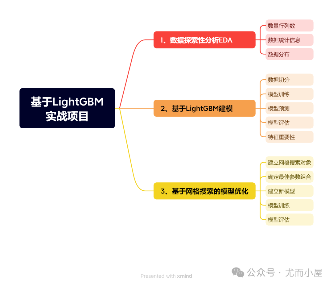
麻雀虽小，五脏俱全

1 导入库

In [1]:

import pandas as pd 
import numpy as np
pd.set_option('display.max_columns', 100)
from IPython.display import display_html


import plotly_express as px
import plotly.graph_objects as go

import matplotlib
import matplotlib.pyplot as plt
plt.rcParams["font.sans-serif"]=["SimHei"] # 设置字体
plt.rcParams["axes.unicode_minus"]=False # 解决“-”负号的乱码问题
import seaborn as sns
%matplotlib inline 

import missingno as ms 
import gc

from datetime import datetime 
from sklearn.model_selection import train_test_split,StratifiedKFold,GridSearchCV
from sklearn.preprocessing import StandardScaler, MinMaxScaler
from sklearn.decomposition import PCA
from imblearn.under_sampling import ClusterCentroids
from imblearn.over_sampling import KMeansSMOTE, SMOTE
from sklearn.model_selection import KFold

from sklearn.metrics import accuracy_score, recall_score, precision_score, f1_score, auc
from sklearn.metrics import roc_auc_score,precision_recall_curve, confusion_matrix,classification_report

# Classifiers
from sklearn.linear_model import LogisticRegression
from sklearn.svm import SVC
from sklearn import tree
from pydotplus import graph_from_dot_data
from sklearn.tree import DecisionTreeClassifier
from sklearn.ensemble import RandomForestClassifier,AdaBoostClassifier
from catboost import CatBoostClassifier
import lightgbm as lgb
import xgboost as xgb

from scipy import stats

import warnings 
warnings.filterwarnings("ignore")

2 数据信息

2.1 导入数据

In [2]:

df = pd.read_csv("信贷数据.csv")

df

Out[2]:

	Income	Age	Sex	History_Credit_Limit	History_Default_Times	Default
0	462087	26	1	0	1	1
1	362324	32	0	13583	0	1
2	332011	52	1	0	1	1
3	252895	39	0	0	1	1
4	352355	50	1	0	0	1
...	...	...	...	...	...	...
995	442985	24	1	5000	0	0
996	402396	39	0	0	0	0
997	442684	36	1	10000	0	0
998	382029	43	1	0	0	0
999	422612	39	0	91040	1	0

1000 rows × 6 columns

2.2 数据基本信息

In [3]:

df.columns

Out[3]:

Index(['Income', 'Age', 'Sex', 'History_Credit_Limit', 'History_Default_Times',
       'Default'],
      dtype='object')

缺失值情况：

In [4]:

df.isnull().sum()

Out[4]:

Income                   0
Age                      0
Sex                      0
History_Credit_Limit     0
History_Default_Times    0
Default                  0
dtype: int64

历史违约次数统计：

In [5]:

df["History_Default_Times"].value_counts()

Out[5]:

History_Default_Times
0    615
1    203
2    129
3     43
4      7
5      3
Name: count, dtype: int64

In [6]:

df["Sex"].value_counts()

Out[6]:

Sex
1    507
0    493
Name: count, dtype: int64

男女人数几乎相同，很均衡。

目标变量是否违约的人数对比：

In [7]:

df["Default"].value_counts()

Out[7]:

Default
0    601
1    399
Name: count, dtype: int64

In [8]:

df[df["History_Default_Times"] == 2]

Out[8]:

	Income	Age	Sex	History_Credit_Limit	History_Default_Times	Default
9	392372	47	1	71000	2	1
12	362640	20	1	0	2	1
13	352044	22	0	0	2	1
14	312971	24	0	0	2	1
18	282051	37	0	63639	2	1
...	...	...	...	...	...	...
941	442329	44	1	28649	2	0
942	392150	57	1	44058	2	0
959	352358	38	1	265208	2	0
991	392087	43	1	236726	2	0
994	342022	20	0	57001	2	0

129 rows × 6 columns

需要注意的是：历史违约次数大于0，不代表一定是违约客户。比如历史违约次数为2，最终是否违约的客户两种情况都有。

是否违约的客户收入存在差异：

In [9]:

fig = px.violin(df, x="Default",y="Income")

fig.show()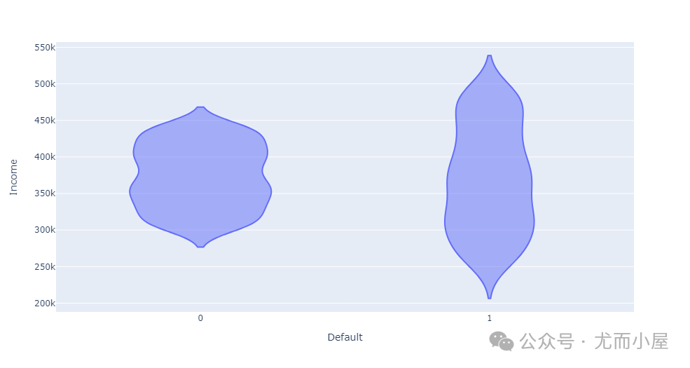

基于seaborn绘制密度图：

In [10]:

sns.displot(data=df,x="Income",hue="Default",kind="kde")

plt.show()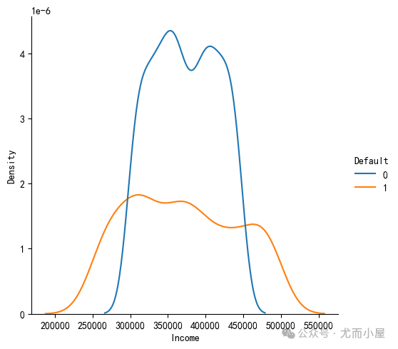

可以看到在低收入和高收入人群中容易发生违约。

In [11]:

fig = px.violin(df, x="Default",y="Age")

fig.show()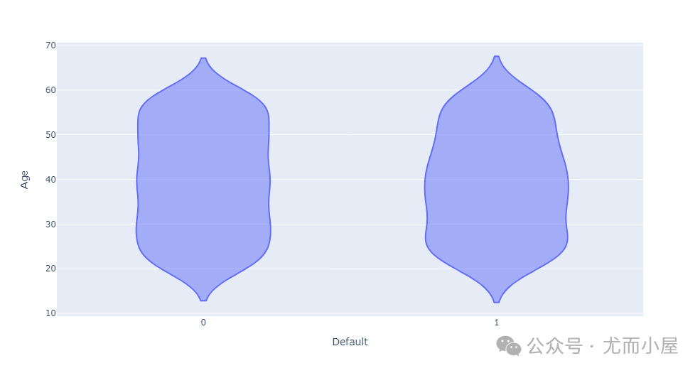

基于seaborn的实现：

In [12]:

sns.displot(data=df,x="Age",hue="Default",kind="kde")

plt.show()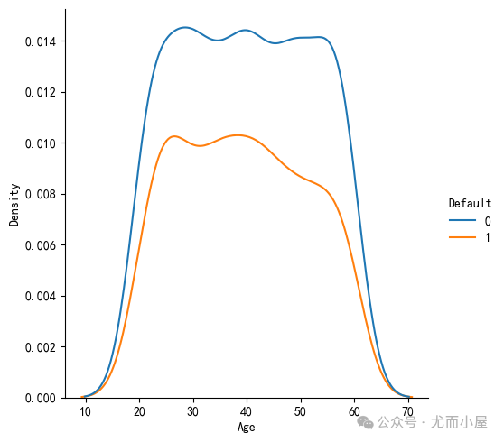

可以看到是是否违约客户的年龄段分布是一致的。

3 LightGBM建模

3.1 切分数据

In [13]:

#  提取特征和目标变量

X = df.drop(columns="Default")
Y = df["Default"]

划分训练集和测试集数据：

In [14]:

from sklearn.model_selection import train_test_split

X_train, X_test, y_train, y_test = train_test_split(X,Y,test_size=0.2,random_state=42)

3.2 模型训练

建立基础版的lightgbm模型：

In [15]:

from lightgbm import LGBMClassifier

model = LGBMClassifier()
model.fit(X_train, y_train)  # 模型训练 
[LightGBM] [Info] Number of positive: 318, number of negative: 482
gain, best gain: -inf
......

Out[15]:

LGBMClassifier

LGBMClassifier()
# 通过下面的代码查看官方解释
LGBMClassifier?

3.3 模型预测

In [16]:

y_pred = model.predict(X_test)
y_pred

Out[16]:

array([0, 0, 0, 0, 0, 0, 0, 0, 0, 1, 0, 0, 0, 0, 1, 0, 1, 0, 1, 0, 0, 1,
       0, 0, 1, 0, 1, 0, 0, 0, 1, 0, 1, 0, 1, 0, 0, 0, 1, 1, 1, 0, 0, 0,
       0, 0, 0, 1, 0, 0, 0, 0, 1, 0, 0, 1, 0, 0, 1, 0, 0, 0, 0, 1, 0, 0,
       0, 0, 0, 0, 0, 0, 0, 0, 1, 1, 0, 1, 0, 1, 0, 1, 1, 1, 0, 0, 0, 0,
       0, 0, 1, 0, 0, 0, 0, 0, 0, 1, 1, 0, 0, 1, 0, 0, 0, 0, 1, 0, 1, 0,
       0, 0, 0, 0, 1, 0, 0, 1, 0, 0, 0, 0, 0, 1, 1, 0, 0, 0, 0, 0, 0, 1,
       1, 0, 0, 1, 1, 1, 1, 1, 1, 1, 0, 1, 0, 0, 0, 0, 0, 1, 0, 1, 0, 0,
       0, 0, 1, 0, 1, 0, 0, 0, 0, 0, 0, 0, 1, 0, 1, 1, 0, 0, 1, 0, 0, 1,
       1, 1, 1, 0, 0, 0, 1, 0, 0, 1, 0, 1, 1, 0, 0, 0, 0, 1, 0, 0, 0, 1,
       0, 0], dtype=int64)

3.4 模型评估

1、对比测试集中的实际值和预测值：

In [17]:

predict_true = pd.DataFrame()

predict_true["预测值"] = list(y_pred)
predict_true["实际值"] = list(y_test)
predict_true

Out[17]:

	预测值	实际值
0	0	0
1	0	0
2	0	0
3	0	0
4	0	0
...	...	...
195	0	0
196	0	1
197	1	1
198	0	0
199	0	1

200 rows × 2 columns

筛选预测值和实际值相等的数据：结果表明是162条记录

In [18]:

predict_true[predict_true["预测值"] == predict_true["实际值"]]

Out[18]:

	预测值	实际值
0	0	0
1	0	0
2	0	0
3	0	0
4	0	0
...	...	...
192	0	0
193	1	1
195	0	0
197	1	1
198	0	0

162 rows × 2 columns

In [19]:

from sklearn.metrics import accuracy_score

accuracy = accuracy_score(y_pred, y_test)
accuracy

Out[19]:

0.81

可以看到模型在测试集上的准确率为81%

也可以计算为：

In [20]:

162 / 200  # 相同数目为162， 总共是200条

Out[20]:

0.81

2、ROC-AUC曲线的绘制：

In [21]:

y_pred_proba = model.predict_proba(X_test)
y_pred_proba[:5]

Out[21]:

array([[0.97884615, 0.02115385],
       [0.99221142, 0.00778858],
       [0.72394845, 0.27605155],
       [0.75366821, 0.24633179],
       [0.95015727, 0.04984273]])

In [22]:

from sklearn.metrics import roc_curve  # ROC-AUC曲线

fpr, tpr, thres = roc_curve(y_test, y_pred_proba[:,1])

In [23]:

plt.plot(fpr, tpr)
plt.title("ROC_AUC Curve of Default")
plt.show()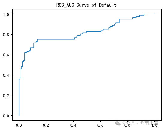

3、查看具体的AUC值：

In [24]:

# 计算AUC的值

from sklearn.metrics import roc_auc_score
score = roc_auc_score(y_test, y_pred_proba[:,1])

score

Out[24]:

0.818290279074593

3.5 特征重要性

In [25]:

# feature_importances_

model.feature_importances_

Out[25]:

array([1179,  668,   96,  906,  131])

In [26]:

model.feature_name_

Out[26]:

['Income', 'Age', 'Sex', 'History_Credit_Limit', 'History_Default_Times']

In [27]:

features = dict(zip(model.feature_importances_,model.feature_name_))
features

Out[27]:

{1179: 'Income',
 668: 'Age',
 96: 'Sex',
 906: 'History_Credit_Limit',
 131: 'History_Default_Times'}

In [28]:

sorted(features.items(),key=lambda x:x[0], reverse=True)

Out[28]:

[(1179, 'Income'),
 (906, 'History_Credit_Limit'),
 (668, 'Age'),
 (131, 'History_Default_Times'),
 (96, 'Sex')]

可以看到基于重要性程度排序后，Income是最重要的，而年龄是最不重要的。

上面的数据信息部分中我们也观察到，是否违约的客户的年龄分布是一致的，也就是说和年龄关系不大。

也可以将特征及其重要性生成DataFrame数据：

In [29]:

features_df = pd.DataFrame({"features": model.feature_name_,"importances": model.feature_importances_})
features_df

Out[29]:

	features	importances
0	Income	1179
1	Age	668
2	Sex	96
3	History_Credit_Limit	906
4	History_Default_Times	131

In [30]:

features_df.sort_values("importances", ascending=False)

Out[30]:

	features	importances
0	Income	1179
3	History_Credit_Limit	906
1	Age	668
4	History_Default_Times	131
2	Sex	96

4 模型调优

基于网格搜索的模型调优：

In [31]:

from sklearn.model_selection import GridSearchCV

4.1 设定网格搜索对象

设定待搜索的参数及其取值范围：

In [32]:

parameters = {"num_leaves": [10, 15, 13],
              "n_estimators":[10,20,30],
              "learning_rate":[0.05,0.1,0.2]
             }

In [33]:

model = LGBMClassifier()  #  基础模型实例化

# 定义搜索实例化对象
grid_search = GridSearchCV(model, # 基础模型
                           parameters,  # 搜索参数
                           scoring="roc_auc", # 评价指标
                           cv=5  # 交叉验证5次
                          )

In [34]:

grid_search.fit(X_train, y_train)  # 模型训练

4.2 建立新模型

输出最佳的参数组合：

In [35]:

dict_params = grid_search.best_params_  

dict_params

Out[35]:

{'learning_rate': 0.05, 'n_estimators': 30, 'num_leaves': 10}

基于最佳的参数组合建立新模型：

In [36]:

new_model = LGBMClassifier(num_leaves=10, # 使用最佳参数
                           n_estimators=30,
                           learning_rate=0.05
                          )

4.3 模型训练

模型再次训练：

In [37]:

new_model.fit(X_train, y_train)
[LightGBM] [Info] Number of positive: 318, number of negative: 482
[LightGBM] [Info] Auto-choosing col-wise multi-threading, the overhead of testing was 0.001194 seconds.
You can set `force_col_wise=true` to remove the overhead.
[LightGBM] [Info] Total Bins 498
[LightGBM] [Info] Number of data points in the train set: 800, number of used features: 5
[LightGBM] [Info] [binary:BoostFromScore]: pavg=0.397500 -> initscore=-0.415893
[LightGBM] [Info] Start training from score -0.415893

4.4 模型评估

1、查看ROC-AUC曲线：

In [38]:

y_pred_proba = new_model.predict_proba(X_test)
y_pred_proba[:5]

Out[38]:

array([[0.77658791, 0.22341209],
       [0.80601961, 0.19398039],
       [0.69243702, 0.30756298],
       [0.7962625 , 0.2037375 ],
       [0.80601961, 0.19398039]])

In [39]:

fpr, tpr, thres = roc_curve(y_test, y_pred_proba[:,1])

plt.plot(fpr, tpr)
plt.title("ROC_AUC Curve of Default")
plt.show()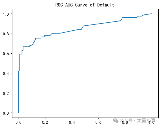

2、具体的AUC值：

In [40]:

# 计算AUC的值

from sklearn.metrics import roc_auc_score
score = roc_auc_score(y_test, y_pred_proba[:,1])

score

Out[40]:

0.8507106546322232

3、再次查看模型的准确率：

In [41]:

# 新模型下的准确率

y_pred_new = new_model.predict(X_test)

accuracy = accuracy_score(y_pred_new, y_test)
accuracy

Out[41]:

0.84

相比较于基础模型的准确率81%，提升了3%

往期精彩回顾




适合初学者入门人工智能的路线及资料下载(图文+视频)机器学习入门系列下载机器学习及深度学习笔记等资料打印《统计学习方法》的代码复现专辑

• 交流群

欢迎加入机器学习爱好者微信群一起和同行交流，目前有机器学习交流群、博士群、博士申报交流、CV、NLP等微信群，请扫描下面的微信号加群，备注：”昵称-学校/公司-研究方向“，例如：”张小明-浙大-CV“。请按照格式备注，否则不予通过。添加成功后会根据研究方向邀请进入相关微信群。请勿在群内发送广告，否则会请出群，谢谢理解~（也可以加入机器学习交流qq群772479961）