用PyG (PyTorch Geometric) 中的MPNN和RDkit构建模型，并预测NCI1中smile分子的致癌性（二分类问题）

一：NCI1 dataset介绍

NCI1数据集来自化学信息学领域，其中每个输入图都用作化合物的表示：每个顶点代表分子的一个原子，顶点之间的边代表原子之间的键。该数据集与抗癌筛查有关，其中化学物质被评估为对细胞肺癌呈阳性或阴性。每个顶点都有一个代表相应原子类型的输入标签，通过单热编码方案编码为 0/1 元素的向量。

它可以在torch_geometric.datasets的TUDataset中直接调用，所以它已经转换成PyG中的图数据格式了，而节点的原子元素不知道是什么，原本smile分子式更不清楚。所以我查了一下原文，顺藤摸瓜找到了出处。论文介绍在：Comparison of descriptor spaces for chemical compound retrieval and classification

在论文中，关于NCI-H23 (NCI1)的描述是Human tumor (Non-small cell lung) cell line growth inhibition assay，查到数据出自：PubChem AID    https://pubchem.ncbi.nlm.nih.gov/bioassay/21

关于它的描述：Growth inhibition of the EKVX human Non-Small Cell Lung tumor cell line is measured as a screen for anti-cancer activity. Cells are grown in 96 well plates and exposed to the test compound for 48 hours. Compounds are tested at 5 different concentrations and three endpoints are estimated from this dose response curve: GI50, concentration required for 50% inhibition of growth, TGI, the concentration requires for complete inhibition of growth, and LC50, the concentration required for 50% reduction in cell number. These estimates are done by simple linear interpolation between the concentrations that surround the approriate level. If a compound doesn't cause inhibition to the appropriate level, the endpoint is set to the highest concentration tested

These data are a subset of the data from the NCI human tumor cell line screen. Compounds are identified by the NCI NSC number. In the NCI numbering system, EKVX is panel number 1, cell number 8

Basically compounds with LogGI50 (unit M) less than -6 were considered as active. Activity score was based on increasing values of -LogGI50

所以，NCI只是其中的一部分数据集，LogGI50 (unit M)小于-6的被认为active，有致癌性。

二：数据集处理

提取smile分子和其对应的activity，其中只选择含有C，H，N，O，F, Cl , Br , I这几种元素的smile分子式。总数据量为9900+，其中inactive和active的比例式5.66：1。出现了样本数据不均衡问题，所以先试着下采样处理一下，强行调到1：1。本文只着重介绍如何训练预测，其结果可能会不尽人意。

三：特征提取

特征提取参考了：Message-passing neural network (MPNN) for molecular property prediction

为了编码原子和键的原子特征。我们将定义两个类：AtomFeaturizer和BondFeaturizer。仅考虑少数（原子和键）特征：[原子特征]符号（元素），价电子，氢键数，轨道杂交，[键特征]（共价）键类型和共轭。将原子各个特征生成one-hot vector 并concate成一个新的向量，边的特征同理。

class Featurizer:
    def __init__(self, allowable_sets):
        self.dim = 0
        self.features_mapping = {}
        for k, s in allowable_sets.items():
            s = sorted(list(s))
            self.features_mapping[k] = dict(zip(s, range(self.dim, len(s) + self.dim)))
            self.dim += len(s)

    def encode(self, inputs):
        output = np.zeros((self.dim,))
        for name_feature, feature_mapping in self.features_mapping.items():
            feature = getattr(self, name_feature)(inputs)
            if feature not in feature_mapping:
                continue
            output[feature_mapping[feature]] = 1.0
        return output


class AtomFeaturizer(Featurizer):
    def __init__(self, allowable_sets):
        super().__init__(allowable_sets)

    def symbol(self, atom):
        return atom.GetSymbol()

    def n_valence(self, atom):
        return atom.GetTotalValence()

    def n_hydrogens(self, atom):
        return atom.GetTotalNumHs()

    def hybridization(self, atom):
        return atom.GetHybridization().name.lower()


class BondFeaturizer(Featurizer):
    def __init__(self, allowable_sets):
        super().__init__(allowable_sets)
        self.dim

    def encode(self, bond):
        output = np.zeros((self.dim,))
        if bond is None:
            output[-1] = 1.0
            return output
        output = super().encode(bond)
        return output

    def bond_type(self, bond):
        return bond.GetBondType().name.lower()

    def conjugated(self, bond):
        return bond.GetIsConjugated()


atom_featurizer = AtomFeaturizer(
    allowable_sets={
        "symbol": {"Br", "C",  "Cl", "F", "H", "I", "N",  "O"},
        "n_valence": {0, 1, 2, 3, 4, 5, 6},
        "n_hydrogens": {0, 1, 2, 3, 4},
        "hybridization": {"s", "sp", "sp2", "sp3"},
    }
)

bond_featurizer = BondFeaturizer(
    allowable_sets={
        "bond_type": {"single", "double", "triple", "aromatic"},
        "conjugated": {True, False},
    }
)

四：MoleculesDataset

生成PyG dataloader要使用的dataset，使用能一次性放入内存的InMemoryDataset类，并存放到文件中，每次运行只需在这个文件里读取就行。只需第一次处理数据，之后都能快读读取，大大提高效率。

class MoleculesDataset(InMemoryDataset):
    def __init__(self, root, transform = None):
        super(MoleculesDataset,self).__init__(root, transform)
        self.data, self.slices = torch.load(self.processed_paths[0])

    @property
    def raw_file_names(self):
        return 'data.csv'

    @property
    def processed_file_names(self):
        return 'data.pt'

    def download(self):
        # Download to `self.raw_dir`.
        pass

    def process(self):
        datas = []
        for smile, y in zip(smiles, ys):
            mol = Chem.MolFromSmiles(smile)
            mol = Chem.AddHs(mol)

            embeddings = []
            for atom in mol.GetAtoms():
                embeddings.append(atom_featurizer.encode(atom))
            embeddings = torch.tensor(embeddings,dtype=torch.float32)

            edges = []
            edge_attr = []
            for bond in mol.GetBonds():
                edges.append([bond.GetBeginAtomIdx(), bond.GetEndAtomIdx()])
                edges.append([bond.GetEndAtomIdx(), bond.GetBeginAtomIdx()])

                edge_attr.append(bond_featurizer.encode(bond))
                edge_attr.append(bond_featurizer.encode(bond))

            edges = torch.tensor(edges).T
            edge_attr = torch.tensor(edge_attr,dtype=torch.float32)

            y = torch.tensor(y, dtype=torch.long)

            data = Data(x=embeddings, edge_index=edges, y=y, edge_attr=edge_attr)
            datas.append(data)

        # self.data, self.slices = self.collate(datas)
        torch.save(self.collate(datas), self.processed_paths[0])

五：数据集划分

train ：val ：test = 8：1：1

train_size = int(0.8 * len(dataset))
valid_size = int(0.1 * len(dataset))
test_size = len(dataset) - train_size - valid_size
train_dataset, valid_dataset, test_dataset = torch.utils.data.random_split(dataset, [train_size,valid_size, test_size],generator=torch.Generator().manual_seed(1))


test_loader = DataLoader(test_dataset, batch_size=128, shuffle=False)
val_loader = DataLoader(valid_dataset, batch_size=128, shuffle=False)
train_loader = DataLoader(train_dataset, batch_size=128, shuffle=True)

六：模型建立

使用torch_geometric.nn自带的NNConv, Set2Set，建立模型，消息传递NNConv过程执行两次。

因为NNConv后处理的数据还是整个图的节点数据，还需要个readout函数将其压缩到一个向量，之后放到MLP中，最后进行二分类。

整个NNConv的整个思路式先将边向量数据放入nn模型，输出能和邻居节点向量做内积的shape后，和邻居节点做内积，再将这些邻居节点的内积和当前节点的向量相加，通过这样子，元素节点聚合了邻居节点和边的信息。

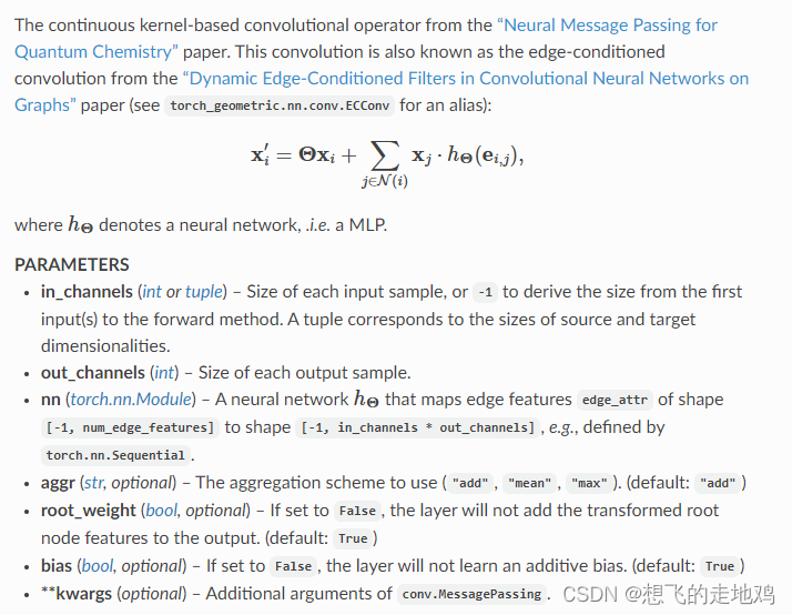
 NNConv的文档

torch_geometric.nn.conv.NNConv — pytorch_geometric documentation

readout函数我使用了它自带的Set2Set。它的论文：《Order Matters: Sequence to sequence for sets》

class NNConvNet(nn.Module):
    def __init__(self,node_feature_dim, edge_feature_dim, edge_hidden_dim):
        super(NNConvNet,self).__init__()
        #第一层
        edge_network1 = nn.Sequential(
            nn.Linear(edge_feature_dim, edge_hidden_dim),
            nn.ReLU(),
            nn.Linear(edge_hidden_dim, node_feature_dim * node_feature_dim)
        )
        self.nnconv1 = NNConv(node_feature_dim, node_feature_dim, edge_network1, aggr="mean")

        # # 第二层
        # edge_network2 = nn.Sequential(
        #     nn.Linear(edge_feature_dim, edge_hidden_dim),
        #     nn.ReLU(),
        #     nn.Linear(edge_hidden_dim, 32 * 16)
        # )
        # self.nnconv2 = NNConv(32, 16, edge_network2, aggr="mean")


        self.relu = nn.ReLU()
        self.set2set = Set2Set(24, processing_steps=3)
        self.fc2 = nn.Linear(2 * 24, 8)
        self.fc3 = nn.Linear(8, 2)

    def forward(self,data):
        x, edge_index, edge_attr,batch = data.x, data.edge_index, data.edge_attr,data.batch
        x = self.nnconv1(x, edge_index, edge_attr)
        x = self.relu(x)
        x = self.nnconv1(x, edge_index, edge_attr)
        x = self.set2set(x, batch)
        x = self.fc2(x)
        x = self.relu(x)
        x = self.fc3(x)

        return x

七：模型训练，预测

for e in tqdm(range(num)):
    print('Epoch {}/{}'.format(e + 1, num))
    print('-------------')
    model.train()
    epoch_loss = []

    train_total = 0
    train_correct = 0

    train_preds = []
    train_trues = []
    #train
    for data in train_loader:
        y = data.y
        optimizer.zero_grad()
        out = model(data)

        # print(y.dtype, out.dtype)

        loss = criterion(out, y)
        loss.requires_grad_(True)
        loss.backward()
        optimizer.step()
        epoch_loss.append(loss.data)

        _, predict = torch.max(out.data, 1)
        train_total += y.shape[0] * 1.0
        train_correct += int((y == predict).sum())

        #评估指标
        train_outputs = out.argmax(dim=1)

        train_preds.extend(train_outputs.detach().cpu().numpy())
        train_trues.extend(y.detach().cpu().numpy())

    epoch_loss = np.average(epoch_loss)
    # scheduler.step(epoch_loss)

    # early_stopping(epoch_loss, model)
    # # 若满足 early stopping 要求
    # if early_stopping.early_stop:
    #     print("Early stopping")
    #     # 结束模型训练
    #     break

    #f1_score
    sklearn_f1 = f1_score(train_trues, train_preds)
    print('train Loss: {:.4f} Acc:{:.4f} f1:{:.4f}'.format(epoch_loss,train_correct/train_total,sklearn_f1))
    tra_loss.append(epoch_loss)
    tra_acc.append(train_correct/train_total)
    print(confusion_matrix(train_trues, train_preds))

    #----------------------------------------------------------valid------------------------------------------------------------
    correct = 0
    total = 0

    valid_preds = []
    valid_trues = []

    with torch.no_grad():
        model.eval()
        for data in val_loader:
            labels = data.y
            outputs = model(data)


            _, predict = torch.max(outputs.data, 1)
            total += labels.shape[0] * 1.0
            correct += int((labels == predict).sum())

            valid_outputs = outputs.argmax(dim=1)
            valid_preds.extend(valid_outputs.detach().cpu().numpy())
            valid_trues.extend(labels.detach().cpu().numpy())

        sklearn_f1 = f1_score(valid_trues, valid_preds)

        print('val Acc: {:.4f} f1:{:.4f}'.format(correct / total,sklearn_f1))
        val_acc.append(correct / total)

        print(confusion_matrix(valid_trues, valid_preds))

八：模型预测

correct = 0
total = 0
test_preds = []
test_trues = []
with torch.no_grad():
    model.eval()
    for data in test_loader:

        labels = data.y
        outputs = model(data)

        _, predict = torch.max(outputs.data, 1)
        total += labels.shape[0] * 1.0
        correct += int((labels == predict).sum())

        test_outputs = outputs.argmax(dim=1)
        test_preds.extend(test_outputs.detach().cpu().numpy())
        test_trues.extend(labels.detach().cpu().numpy())

    sklearn_f1 = f1_score(test_trues, test_preds)

    print('test Acc: {:.4f} f1:{:.4f}'.format(correct/total,sklearn_f1))

九：结果评估

结果有点惨，loss是在下降了，但是准确度只有0.66左右。f1_score也不高

分析一波：

1.数据问题，样本少，样本不均很，就算下采样，也无法得到比较好的结果。有一种可能是，测试集和训练集的样本空间本身就不太一样，或者说是测试集有很多和训练集不相似的样本，这是训练样本本身的缺陷问题，这个时候需要额外扩增数据集、

2.有些smile分子式很长，图也很到，图与图之间大小出入很大，将这些图压缩成数据，并训练预测。可能现在的数据式原本样本空间的一小部分，应还是扩增数据集，样本的空间保留原来的多样性。

十：整体代码

https://github.com/sudehong/Predicting-Molecular-Carcinogenicity-By-Using-NCI1-Data

学术技术无界限，如有疑问，欢迎一起探讨。