


目录
资料
深度聚类算法研究综述(很赞,从聚类方法和深度学习方法两个方面进行了总结,我这个可能作为综述前的一篇文章,要是捋出头绪也写一写):https://www.cnblogs.com/kailugaji/p/15574267.html
对比学习代码库:https://github.com/HobbitLong/PyContrast?tab=readme-ov-file
SwAV
论文:https://arxiv.org/pdf/2006.09882
代码:https://github.com/facebookresearch/swav
视频(像我一样的小白必看):https://www.bilibili.com/video/BV1754y187Ki/?spm_id_from=333.337.search-card.all.click
问题
现有的方法通常是在线工作的,依赖于大量的显示的成对特征的比较,在计算上是有挑战性的。
方法
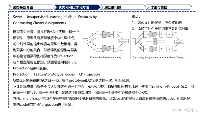
提出了SwAV,不需要成对进行比较。方法同时对数据进行聚类,同时价钱同一图像不同增强之间的一致性,不是像对比学习一样直接表示特征。
提出了新的数据增强multi-crop,在不增加内存或计算需求的情况下,使用不同分辨率的视图混合代替两个全分辨率视图。
方法的创新点
不需要进行成对比较。
我们的方法是内存有效的,就是不需要大的memory bank或者特殊的动量网络。
为什么有效
L
(
z
t
,
z
s
)
=
l
(
z
t
,
q
s
)
+
l
(
z
s
,
q
t
)
,
L(zt, zs) =\mathscr{l}(z_t, q_s) +\mathscr{l}(z_s, q_t),
L(zt,zs)=l(zt,qs)+l(zs,qt),
通过将一组特征匹配到一组K个原型中来计算他们的code
q
t
,
q
s
q_t,q_s
qt,qs。
假设:两个特征包含相同的信息,那么是可以通过其中一个feature去预测另一个的code的。

有什么可以借鉴的地方
聚类
聚类前的特征先投影到单位球面上得到
z
n
t
z_{nt}
znt。
然后把
z
n
t
z_{nt}
znt映射到K个可训练的原型向量上,得到
c
o
d
e
code
code。
如何计算code
SwAV的损失建立了从feature
z
s
z_s
zs到预测code
q
t
q_t
qt,从
z
t
z_t
zt到预测code
q
s
q_s
qs的交换预测的问题。损失是CE Loss,是计算的code和
z
i
z_i
zi和所有在
C
C
C中的原型之间的点积计算softmax得到的概率值。
l
(
z
t
,
q
s
)
=
−
∑
k
q
s
(
k
)
log
p
t
(
k
)
l(z_t, q_s) = − \sum\limits_{k} q_s^{(k)} \log p^{(k)}_t
l(zt,qs)=−k∑qs(k)logpt(k)
where
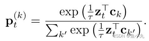
p
t
(
k
)
p^{(k)}_t
pt(k)是第t个feature
z
t
z_t
zt与第k个clusterinng centroid
c
k
c_k
ck进行乘积然后乘以
1
τ
\frac{1}{τ}
τ1计算softmax。
下面这个式子是把展开后的
p
t
(
k
)
p^{(k)}_t
pt(k)带入到损失中,然后拆开得到的,前面两个是分子,后面是分母。

原型C的跨批次使用,SwAV将多个实例聚类到原型。使得同一个批次中所有的样本都被原型等分。约束了不同图像的编码是不同的,避免了每个图像都有相同编码的平凡解。
使用Q矩阵把特征映射到原型,优化Q来最大化特征和原型之间的相似性。
max
Q
∈
Q
T
r
(
Q
T
C
T
Z
)
+
ε
H
(
Q
)
,
\max\limits_{Q∈Q} Tr (Q^TC^TZ) + εH(Q),
Q∈QmaxTr(QTCTZ)+εH(Q),
H(·)是熵,控制映射是平滑的,但是强的熵正则化会导致平凡解,模型会坍塌,所以保持
ε
ε
ε要小。
对Q矩阵进行约束。
Q
=
{
Q
∈
R
+
K
×
B
+
∣
Q
1
B
=
1
K
1
K
,
Q
T
1
K
=
1
B
1
B
}
,
Q= \{ Q ∈ R^{K×B}_{+} + | Q_{1B} = \frac{1}{K} 1_K , Q^T1_K = \frac{1}{B} 1_B \} ,
Q={Q∈R+K×B+∣Q1B=K11K,QT1K=B11B},
式中:1K表示K维向量。这些约束要求批次中平均每个原型至少被选择B K次。使用连续的Q*,不进行离散化,因为获得离散码所需的舍入是比梯度更新更激进的优化步骤。在使模型快速收敛的同时,却导致了更差的解。
在集合Q上,取正规化指数矩阵的形式。
Q
∗
=
D
i
a
g
(
u
)
e
x
p
(
C
T
Z
ε
)
D
i
a
g
(
v
)
,
Q^* = Diag(u) exp( \frac{C^TZ}{ε} ) Diag(v),
Q∗=Diag(u)exp(εCTZ)Diag(v),
其中u和v分别是RK和RB中的重整化向量。重整化向量通过使用迭代的Sinkhorn - Knopp算法,使用少量的矩阵乘法来计算。思考一下u,v怎么整的,我记得代码中有Sinkhorn - Knopp算法。
我们可以使用小批量数据。如果batchsize太小,我们使用之前批次的特征来增加Prob中Z的大小。我们在训练损失中只使用了批特征的编码。
Multi-crop
正如先前的工作所指出的那样,通过捕获场景或对象部分之间的关系信息,比较图像中的随机裁剪起着核心作用。
为了保证内存大小保持不变,有两个高分辨率的裁剪图像,和一些低分辨率(小的)裁剪图像。我们计算code的时候只计算两个高分辨率的图像。计算损失的时候,是用其他图像的特征分别去预测两个高分辨率的特征得到的损失。
L
(
z
t
1
,
z
t
2
,
.
.
.
,
z
t
V
+
2
)
=
∑
i
∈
1
,
2
∑
v
=
1
V
+
2
1
v
≠
i
l
(
z
t
v
,
q
t
i
)
.
L(z_{t_1} , z_{t_2} , . . . , z_{t_{V +2}} ) = \sum\limits_{i∈{1,2}} \sum\limits_{v=1}^{V +2}1_{v\neq i}l(z_{t_v} , q_{t_i} ).
L(zt1,zt2,...,ztV+2)=i∈1,2∑v=1∑V+21v=il(ztv,qti).
代码
下面是训练阶段的代码主要是计算指定的裁剪id的图片计算聚类分配q(也就是文章中的Q)。然后其他所有的裁剪id计算z经过预测头得到的输出p(下面变量中的out)。计算q和out的一致性损失。
def train(train_loader, model, optimizer, epoch, lr_schedule, queue):
    batch_time = AverageMeter()
    data_time = AverageMeter()
    losses = AverageMeter()
    # 创建用于记录批次时间、数据加载时间和损失的对象
    model.train()
    # 将模型设为训练模式
    use_the_queue = False
    # 队列使用标志
    end = time.time()
    for it, inputs in enumerate(train_loader):
        # measure data loading time
        data_time.update(time.time() - end)

        # update learning rate
        iteration = epoch * len(train_loader) + it
        for param_group in optimizer.param_groups:
            param_group["lr"] = lr_schedule[iteration]#是不是两个值

        # normalize the prototypes
        with torch.no_grad():#对原型向量进行归一化
            w = model.module.prototypes.weight.data.clone()
            w = nn.functional.normalize(w, dim=1, p=2)
            model.module.prototypes.weight.copy_(w)

        # ============ multi-res forward passes ... ============
        embedding, output = model(inputs)#得到输出
        embedding = embedding.detach()
        bs = inputs[0].size(0)
        #多尺度前向传播,得到embedding和output,分离嵌入,这个嵌入是做什么的呢,这个嵌入为啥要detach()
        # ============ swav loss ... ============
        loss = 0
        for i, crop_id in enumerate(args.crops_for_assign):#遍历指定的裁剪的图像,也就是两个分辨率大的哪个,对每个裁剪计算输出
            with torch.no_grad():
                out = output[bs * crop_id: bs * (crop_id + 1)].detach()#思考一下,这个就是指定的id的图像的位置,这些裁剪的id的图像长度为bs

                # time to use the queue
                """
                如果队列不为空,并且使用队列或队列已满,则将队列中的嵌入与当前输出拼接。
                更新队列,移动旧的嵌入,并插入新的嵌入。
                """
                if queue is not None:#为什么使用queue?
                    if use_the_queue or not torch.all(queue[i, -1, :] == 0):
                        use_the_queue = True
                        out = torch.cat((torch.mm(
                            queue[i],#Q#相乘是计算相似度吗
                            model.module.prototypes.weight.t()#C
                        ), out))
                    # fill the queue
                    queue[i, bs:] = queue[i, :-bs].clone()#移动
                    queue[i, :bs] = embedding[crop_id * bs: (crop_id + 1) * bs]#crop_id是一个数吧

                # get assignments获取聚类分配。
                q = distributed_sinkhorn(out)[-bs:]#这个是获得q这个是聚类分配的q
                #计算SwAV损失,遍历所有裁剪图像,计算输出和聚类分配之间的交叉熵损失。
            # cluster assignment prediction
            subloss = 0
            for v in np.delete(np.arange(np.sum(args.nmb_crops)), crop_id):#这个才是每一个裁剪图像
                x = output[bs * v: bs * (v + 1)] / args.temperature
                subloss -= torch.mean(torch.sum(q * F.log_softmax(x, dim=1), dim=1))#聚类和输出进行损失计算。
            loss += subloss / (np.sum(args.nmb_crops) - 1)
        loss /= len(args.crops_for_assign)

        # ============ backward and optim step ... ============
        optimizer.zero_grad()
        if args.use_fp16:
            with apex.amp.scale_loss(loss, optimizer) as scaled_loss:
                scaled_loss.backward()
        else:
            loss.backward()
        # cancel gradients for the prototypes
        if iteration < args.freeze_prototypes_niters:
            for name, p in model.named_parameters():
                if "prototypes" in name:
                    p.grad = None
        optimizer.step()

        # ============ misc ... ============
        losses.update(loss.item(), inputs[0].size(0))
        batch_time.update(time.time() - end)
        end = time.time()
        if args.rank ==0 and it % 50 == 0:
            logger.info(
                "Epoch: [{0}][{1}]\t"
                "Time {batch_time.val:.3f} ({batch_time.avg:.3f})\t"
                "Data {data_time.val:.3f} ({data_time.avg:.3f})\t"
                "Loss {loss.val:.4f} ({loss.avg:.4f})\t"
                "Lr: {lr:.4f}".format(
                    epoch,
                    it,
                    batch_time=batch_time,
                    data_time=data_time,
                    loss=losses,
                    lr=optimizer.optim.param_groups[0]["lr"],
                )
            )
    return (epoch, losses.avg), queue
下面这个是计算的聚类分配的代码。
@torch.no_grad()#优化原型分配Q是将feature映射到C的一个函数
def distributed_sinkhorn(out):#这个是最有最优传输的
    Q = torch.exp(out / args.epsilon).t() # Q is K-by-B for consistency with notations from our paper
    #计算输入张量out的指数并进行转置,得到一个大小为K*B的矩阵
    # 计算总的样本数量B
    B = Q.shape[1] * args.world_size # number of samples to assign
    # K是原型的数量,即Q矩阵的行数
    K = Q.shape[0] # how many prototypes

    # make the matrix sums to 1
    sum_Q = torch.sum(Q)
    dist.all_reduce(sum_Q)
    Q /= sum_Q

    for it in range(args.sinkhorn_iterations):#迭代这些次数
        # normalize each row: total weight per prototype must be 1/K
        sum_of_rows = torch.sum(Q, dim=1, keepdim=True)
        dist.all_reduce(sum_of_rows)
        Q /= sum_of_rows
        Q /= K

        # normalize each column: total weight per sample must be 1/B
        Q /= torch.sum(Q, dim=0, keepdim=True)
        Q /= B

    Q *= B # the colomns must sum to 1 so that Q is an assignment
    return Q.t()
resnet代码中添加了原型头和预测头。
PCL
论文:https://arxiv.org/pdf/2005.04966
代码:https://github.com/salesforce/PCL
A prototype is define as “a representative embedding for a group of semantically similar instance”.#原型的定义是全篇的精髓,也是紧紧围绕的中心。
这篇文章是用原型做对比学习。
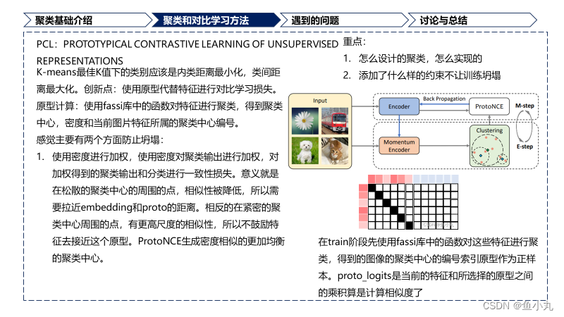
K-means最佳K值下的类别应该是类内距离最小化类间距离最大化

无监督视觉表示学习的任务是学习一个 embedding 函数把
x
x
x 映射到
v
=
{
v
1
,
v
2
,
…
,
v
n
}
v = \{v_1, v2, … ,v_n \}
v={v1,v2,…,vn},其中
v
i
=
f
θ
(
x
i
)
v_i = f_{\theta}(x_i)
vi=fθ(xi)。
本文使用prototyprs
c
c
c 取代
v
′
v'
v′,并且使用每个prototype的密度估计
ϕ
\phi
ϕ代替固定的温度系数
τ
\tau
τ,所以设计了一个原型的对比学习损失。这个是一个创新点。
使用所有特征到原型的距离的二范数来度量密度。
意义就是在松散的聚类中心的周围的点,相似性被降低,所以需要拉近embedding和proto的距离。
相反的在紧密的聚类中心周围的点,有更高尺度的相似性,所以不鼓励特征去接近这个原型。
ProtoNCE生成密度相似的更加均衡的聚类中心。
后面就是把这个方法套入到EM算法中,和EM算法的推导几乎一模一样。感兴趣的可以看EM算法的推导。https://zhuanlan.zhihu.com/p/36331115
最后一个是互信息的进行分析。这里主要是从互信息的角度解释了为什么Proto NCE由于Info NCE。
主要有以下几个优点:
1. Proto NCE忽略了个体的noise,能够获得更加高水平的语义特征。
2. 与Info NCE相比,原型与标签之间存在更大的互信息。这些得益于有效的聚类。
代码
主要使用了fassi库中的clus进行聚类。在Moco的代码上进行修改。
模型代码前面和Moco相同,主要是后面使用了输入的聚类相关信息与特征进行
主要理解下面这段代码就行。
在train阶段先使用fassi库中的函数对这些特征进行聚类,得到的图像的聚类中心的编号索引原型作为正样本。proto_logits是当前的特征和所选择的原型之间的乘积算是计算相似度了。刚开始不明白的点是为什么label是使用linspace进行生成的,侧面是样本,上面是聚类中心的话,我们选择的pos_proto是按照每个样本索引获得的原型的索引,根据原型的索引的到的原型作为正样本,所以标签是linspace得到的没问题。然后还有一点就是它的密度。因为它的这个”密度“的衡量是特征到聚类中心的距离的二范数得到的,所以这个数越大,密度越小,这个数越小密度越大,作为分母,”密度“越大,然后logit值越小,与label之间的差距越大,loss高就迫使模型给它拉近。我的猜测。
        if cluster_result is not None:
            #如果提供了聚类结果,则执行以下代码块。
            proto_labels = []
            proto_logits = []
            for n, (im2cluster,prototypes,density) in enumerate(zip(cluster_result['im2cluster'],cluster_result['centroids'],cluster_result['density'])):
                # get positive prototypes
                pos_proto_id = im2cluster[index]#得看看这个im2cluster和prototypes是怎么合在一起的
                pos_prototypes = prototypes[pos_proto_id]
                #初始化原型标签和对数几率的列表,并遍历聚类结果。
                # sample negative prototypes
                #获取正样本的原型ID和对应的原型。
                all_proto_id = [i for i in range(im2cluster.max()+1)]#
                neg_proto_id = set(all_proto_id)-set(pos_proto_id.tolist())#剩下的就是负的原型
                neg_proto_id = sample(neg_proto_id,self.r) #sample r negative prototypes
                neg_prototypes = prototypes[neg_proto_id]  #这些就是负的原型
                #采样负样本的原型。
                proto_selected = torch.cat([pos_prototypes,neg_prototypes],dim=0)#选择的原型

                # compute prototypical logits
                logits_proto = torch.mm(q,proto_selected.t())#q就是当前得到的特征

                # targets for prototype assignment
                labels_proto = torch.linspace(0, q.size(0)-1, steps=q.size(0)).long().cuda()##这些是聚类的label

                # scaling temperatures for the selected prototypes
                temp_proto = density[torch.cat([pos_proto_id,torch.LongTensor(neg_proto_id).cuda()],dim=0)]#
                logits_proto /= temp_proto #

                proto_labels.append(labels_proto)
                proto_logits.append(logits_proto)
            return logits, labels, proto_logits, proto_labels
        else:
            return logits, labels, None, None
下面是完整的模型的代码。
import torch
import torch.nn as nn
from random import sample

class MoCo(nn.Module):
    """
    Build a MoCo model with: a query encoder, a key encoder, and a queue
    https://arxiv.org/abs/1911.05722
    """
    def __init__(self, base_encoder, dim=128, r=16384, m=0.999, T=0.1, mlp=False):
        """
        dim: feature dimension (default: 128)
        r: queue size; number of negative samples/prototypes (default: 16384)
        m: momentum for updating key encoder (default: 0.999)
        T: softmax temperature
        mlp: whether to use mlp projection
        """
        super(MoCo, self).__init__()

        self.r = r
        self.m = m
        self.T = T

        # create the encoders
        # num_classes is the output fc dimension
        self.encoder_q = base_encoder(num_classes=dim)
        self.encoder_k = base_encoder(num_classes=dim)

        if mlp:  # hack: brute-force replacement
            dim_mlp = self.encoder_q.fc.weight.shape[1]
            self.encoder_q.fc = nn.Sequential(nn.Linear(dim_mlp, dim_mlp), nn.ReLU(), self.encoder_q.fc)
            self.encoder_k.fc = nn.Sequential(nn.Linear(dim_mlp, dim_mlp), nn.ReLU(), self.encoder_k.fc)

        for param_q, param_k in zip(self.encoder_q.parameters(), self.encoder_k.parameters()):
            param_k.data.copy_(param_q.data)  # initialize
            param_k.requires_grad = False  # not update by gradient

        # create the queue
        self.register_buffer("queue", torch.randn(dim, r))#使用了队列,队列里面是特征吗
        self.queue = nn.functional.normalize(self.queue, dim=0)

        self.register_buffer("queue_ptr", torch.zeros(1, dtype=torch.long))

    @torch.no_grad()
    def _momentum_update_key_encoder(self):#动量更新
        """
        Momentum update of the key encoder
        """
        for param_q, param_k in zip(self.encoder_q.parameters(), self.encoder_k.parameters()):
            param_k.data = param_k.data * self.m + param_q.data * (1. - self.m)

    @torch.no_grad()
    def _dequeue_and_enqueue(self, keys):
        # gather keys before updating queue
        keys = concat_all_gather(keys)

        batch_size = keys.shape[0]

        ptr = int(self.queue_ptr)
        assert self.r % batch_size == 0  # for simplicity

        # replace the keys at ptr (dequeue and enqueue)
        self.queue[:, ptr:ptr + batch_size] = keys.T
        ptr = (ptr + batch_size) % self.r  # move pointer

        self.queue_ptr[0] = ptr

    @torch.no_grad()
    def _batch_shuffle_ddp(self, x):
        """
        Batch shuffle, for making use of BatchNorm.
        *** Only support DistributedDataParallel (DDP) model. ***
        """
        # gather from all gpus
        batch_size_this = x.shape[0]
        x_gather = concat_all_gather(x)
        batch_size_all = x_gather.shape[0]

        num_gpus = batch_size_all // batch_size_this

        # random shuffle index
        idx_shuffle = torch.randperm(batch_size_all).cuda()

        # broadcast to all gpus
        torch.distributed.broadcast(idx_shuffle, src=0)

        # index for restoring
        idx_unshuffle = torch.argsort(idx_shuffle)

        # shuffled index for this gpu
        gpu_idx = torch.distributed.get_rank()
        idx_this = idx_shuffle.view(num_gpus, -1)[gpu_idx]

        return x_gather[idx_this], idx_unshuffle

    @torch.no_grad()
    def _batch_unshuffle_ddp(self, x, idx_unshuffle):
        """
        Undo batch shuffle.
        *** Only support DistributedDataParallel (DDP) model. ***
        """
        # gather from all gpus
        batch_size_this = x.shape[0]
        x_gather = concat_all_gather(x)
        batch_size_all = x_gather.shape[0]

        num_gpus = batch_size_all // batch_size_this

        # restored index for this gpu
        gpu_idx = torch.distributed.get_rank()
        idx_this = idx_unshuffle.view(num_gpus, -1)[gpu_idx]

        return x_gather[idx_this]

    def forward(self, im_q, im_k=None, is_eval=False, cluster_result=None, index=None):
        """
        Input:
            im_q: a batch of query images
            im_k: a batch of key images
            is_eval: return momentum embeddings (used for clustering)
            cluster_result: cluster assignments, centroids, and density
            index: indices for training samples
        Output:
            logits, targets, proto_logits, proto_targets
        """

        if is_eval:
            k = self.encoder_k(im_q)
            k = nn.functional.normalize(k, dim=1)
            return k

        # compute key features
        with torch.no_grad():  # no gradient to keys
            self._momentum_update_key_encoder()  # update the key encoder

            # shuffle for making use of BN
            im_k, idx_unshuffle = self._batch_shuffle_ddp(im_k)

            k = self.encoder_k(im_k)  # keys: NxC
            k = nn.functional.normalize(k, dim=1)

            # undo shuffle
            k = self._batch_unshuffle_ddp(k, idx_unshuffle)

        # compute query features
        q = self.encoder_q(im_q)  # queries: NxC
        q = nn.functional.normalize(q, dim=1)

        # compute logits
        # Einstein sum is more intuitive
        # positive logits: Nx1
        l_pos = torch.einsum('nc,nc->n', [q, k]).unsqueeze(-1)
        # negative logits: Nxr
        l_neg = torch.einsum('nc,ck->nk', [q, self.queue.clone().detach()])#k个原型,每个是c维度

        # logits: Nx(1+r)
        logits = torch.cat([l_pos, l_neg], dim=1)

        # apply temperature
        logits /= self.T

        # labels: positive key indicators
        labels = torch.zeros(logits.shape[0], dtype=torch.long).cuda()

        # dequeue and enqueue
        self._dequeue_and_enqueue(k)
        #下面这个就属于空白区域了
        # prototypical contrast
        if cluster_result is not None:
            #如果提供了聚类结果,则执行以下代码块。
            proto_labels = []
            proto_logits = []
            for n, (im2cluster,prototypes,density) in enumerate(zip(cluster_result['im2cluster'],cluster_result['centroids'],cluster_result['density'])):
                # get positive prototypes
                pos_proto_id = im2cluster[index]#得看看这个im2cluster和prototypes是怎么合在一起的
                pos_prototypes = prototypes[pos_proto_id]
                #初始化原型标签和对数几率的列表,并遍历聚类结果。
                # sample negative prototypes
                #获取正样本的原型ID和对应的原型。
                all_proto_id = [i for i in range(im2cluster.max()+1)]#
                neg_proto_id = set(all_proto_id)-set(pos_proto_id.tolist())#剩下的就是负的原型
                neg_proto_id = sample(neg_proto_id,self.r) #sample r negative prototypes
                neg_prototypes = prototypes[neg_proto_id]  #这些就是负的原型
                #采样负样本的原型。
                proto_selected = torch.cat([pos_prototypes,neg_prototypes],dim=0)#选择的原型

                # compute prototypical logits
                logits_proto = torch.mm(q,proto_selected.t())#q就是当前得到的特征

                # targets for prototype assignment
                labels_proto = torch.linspace(0, q.size(0)-1, steps=q.size(0)).long().cuda()##这些是聚类的label

                # scaling temperatures for the selected prototypes
                temp_proto = density[torch.cat([pos_proto_id,torch.LongTensor(neg_proto_id).cuda()],dim=0)]#
                logits_proto /= temp_proto #

                proto_labels.append(labels_proto)
                proto_logits.append(logits_proto)
            return logits, labels, proto_logits, proto_labels
        else:
            return logits, labels, None, None
值得学习的地方我感觉就是这个run_kmeans聚类了,调用了fassi库。
def run_kmeans(x, args):#就是使用faiss库中的函数完成的聚类。
    """
    Args:
        x: data to be clustered
    """

    print('performing kmeans clustering')
    results = {'im2cluster':[],'centroids':[],'density':[]}#初始化一个字典用来存储聚类结果

    for seed, num_cluster in enumerate(args.num_cluster):#遍历聚类中心
        # intialize faiss clustering parameters
        d = x.shape[1]#获取x的维度d应该x就是个二维的
        k = int(num_cluster)
        clus = faiss.Clustering(d, k)#创建一个聚类对象,指定数据维度和聚类数量
        clus.verbose = True
        clus.niter = 20#迭代次数为20
        clus.nredo = 5#重新聚类次数为5
        clus.seed = seed
        clus.max_points_per_centroid = 1000#每个中心点的最大样本数
        clus.min_points_per_centroid = 10

        res = faiss.StandardGpuResources()#初始化聚类资源
        cfg = faiss.GpuIndexFlatConfig()#创建gpu索引配置
        cfg.useFloat16 = False
        cfg.device = args.gpu
        index = faiss.GpuIndexFlatL2(res, d, cfg)#创建一个L2位置索引

        clus.train(x, index) #利用clus对象在index上训练数据x

        D, I = index.search(x, 1) # for each sample, find cluster distance and assignments搜索数据'x'找到每个样本的聚类距离D和分配r
        im2cluster = [int(n[0]) for n in I]#转换成列表每个元素对应一个样本所属的聚类

        # get cluster centroids
        centroids = faiss.vector_to_array(clus.centroids).reshape(k,d)#获取聚类中心点,将其转换成numpy数组

        # sample-to-centroid distances for each cluster
        Dcluster = [[] for c in range(k)]#初始化一个列表用于存储每个聚类的样本距离
        for im,i in enumerate(im2cluster):
            Dcluster[i].append(D[im][0])

        # concentration estimation (phi)
        density = np.zeros(k)#density初始化为0数组
        for i,dist in enumerate(Dcluster):#计算密度,是距离的开根号然后取平均
            if len(dist)>1:#计算每个聚类的密度,如果聚类中样本数大于 1,则计算距离的均值并进行缩放。
                d = (np.asarray(dist)**0.5).mean()/np.log(len(dist)+10)
                density[i] = d

        #if cluster only has one point, use the max to estimate its concentration
        dmax = density.max()#获取最大密度 dmax。
        for i,dist in enumerate(Dcluster):#对于只有一个样本的聚类,使用 dmax 作为其密度。
            if len(dist)<=1:
                density[i] = dmax

        density = density.clip(np.percentile(density,10),np.percentile(density,90)) #clamp extreme values for stability
        #对密度进行裁剪,限制在第 10 和第 90 百分位之间。
        density = args.temperature*density/density.mean()  #scale the mean to temperature 将密度缩放到指定温度 args.temperature。

        # convert to cuda Tensors for broadcast
        centroids = torch.Tensor(centroids).cuda()
        centroids = nn.functional.normalize(centroids, p=2, dim=1)

        im2cluster = torch.LongTensor(im2cluster).cuda()
        density = torch.Tensor(density).cuda()
        #将每个聚类的结果添加到 results 字典中。
        results['centroids'].append(centroids)
        results['density'].append(density)
        results['im2cluster'].append(im2cluster)

    return results
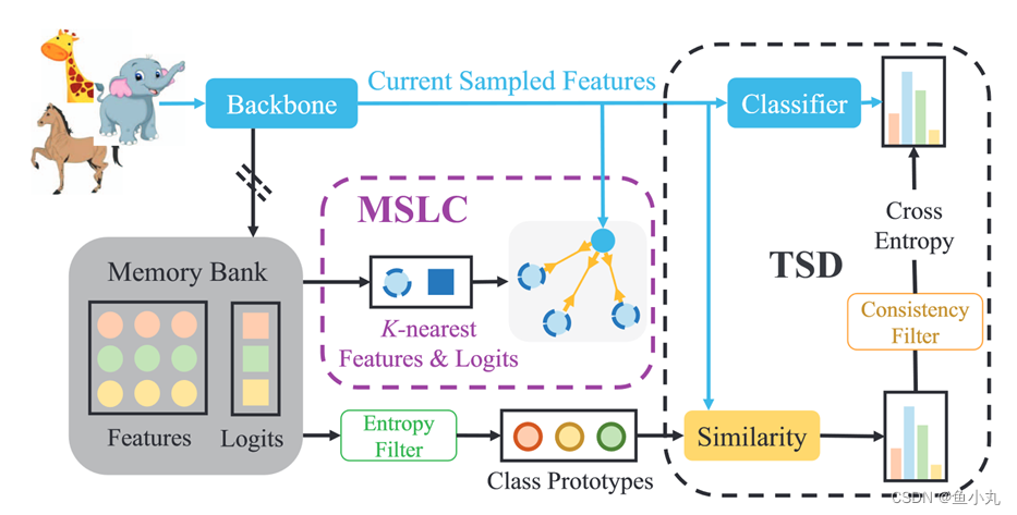
Feature Alignment and Uniformity for Test Time Adaptation
这个是我接触的第一篇我搞懂一点的聚类。
这个就是直接的feature聚类。
第一次将TTA作为特征修订问题来解决。
代码
主体代码如下:
本文主要有两个任务:
一个是一致性任务:计算两个输出之间的一致性损失主要代码在 def prototype_loss(self,z,p,labels=None,use_hard=False,tau=1)这个函数中,然后其中z是特征,p是weights =
s
u
p
p
o
r
t
s
T
supports^T
supportsTlabels这个是支持特征与score之间对应的矩阵,dist =
z
∗
p
T
z *p^T
z∗pT意思就是将当前样本的特征与这个weights(代码中的p)相乘得到BK的值,也就是dist作为聚类任务的输出。labels经过argmax得到硬标签。
另一个是对齐,更新聚类中心。在topk_cluster这个函数中,z.detach().clone()特征supports支持的特征memory中保存的,self.scores得分,p是分类头输出,k是几个近邻。
先进行归一化,然后用特征计算相似度矩阵,选k个最相似的score与p计算差值平方作为距离,
loss = -sim_matrix*diff_scores越接近,最后输出应该越相似。
class TSD(nn.Module):
    """
    Test-time Self-Distillation (TSD)
    CVPR 2023
    """
    def __init__(self,model,optimizer,lam=0,filter_K=100,steps=1,episodic=False):
        super().__init__()
        self.model = model
        self.featurizer = model.featurizer#这个是进行特征提取
        self.classifier = model.classifier#分类头
        self.optimizer = optimizer
        self.steps = steps
        assert steps > 0, "requires >= 1 step(s) to forward and update"
        self.episodic = episodic#是否是记忆的
        self.filter_K = filter_K#选择的支持样本的数量

        warmup_supports = self.classifier.fc.weight.data.detach()#获取分类头的权重
        self.num_classes = warmup_supports.size()[0]#获取类别的数量
        self.warmup_supports = warmup_supports#这个是进行初始化
        warmup_prob = self.classifier(self.warmup_supports)#获取分类头的输出

        self.warmup_ent = softmax_entropy(warmup_prob)#这个是计算熵值#
        self.warmup_labels = F.one_hot(warmup_prob.argmax(1), num_classes=self.num_classes).float()#获取预测的标签,然后one-hot编码
        self.warmup_scores = F.softmax(warmup_prob,1)#

        self.supports = self.warmup_supports.data#这个是进行初始化,
        self.labels = self.warmup_labels.data
        self.ent = self.warmup_ent.data
        self.scores = self.warmup_scores.data
        self.lam = lam


    def forward(self,x):
        z = self.featurizer(x)
        p = self.classifier(z)#模型预测

        yhat = F.one_hot(p.argmax(1), num_classes=self.num_classes).float()#得到的预测标签
        ent = softmax_entropy(p)#计算熵值,用来进行过滤⭐⭐⭐
        scores = F.softmax(p,1)#计算概率⭐⭐⭐
        #如果可以我可以直接用这个代码,
        #概率值的分布,scores进行概率更新
        with torch.no_grad():
            self.supports = self.supports.to(z.device)
            self.labels = self.labels.to(z.device)
            self.ent = self.ent.to(z.device)
            self.scores = self.scores.to(z.device)#移动到当前设备上
            self.supports = torch.cat([self.supports,z])#为什么都合并起来
            self.labels = torch.cat([self.labels,yhat])
            self.ent = torch.cat([self.ent,ent])#熵值
            self.scores = torch.cat([self.scores,scores])

            supports, labels = self.select_supports()#选择,是不是保持支持样本的数量,合并起来是为了更新,然后选择就是进行更新
            supports = F.normalize(supports, dim=1)#归一化
            weights = (supports.T @ (labels))#计算权重,是不是就是那个把概率当成权值,然后对feature进行加权求和

        dist,loss = self.prototype_loss(z,weights.T,scores,use_hard=False)

        loss_local = topk_cluster(z.detach().clone(),supports,self.scores,p,k=3)#计算损失
        loss += self.lam*loss_local#加上一个正则项
        self.optimizer.zero_grad()
        loss.backward()
        self.optimizer.step()
        return p

    def select_supports(self):
        ent_s = self.ent#获取样本的熵值,根据熵值来进行样本选择?
        y_hat = self.labels.argmax(dim=1).long()#从对象的标签属性中获得预测的标签,以及类别索引
        filter_K = self.filter_K#这个是支持的样本数量
        if filter_K == -1:#如果filter_K=-1,那么就是所有的样本
            indices = torch.LongTensor(list(range(len(ent_s))))#获得indice

        indices = []#这个是
        indices1 = torch.LongTensor(list(range(len(ent_s)))).cuda()
        for i in range(self.num_classes):#对每一个类别进行操作
            _, indices2 = torch.sort(ent_s[y_hat == i])#对当前类别的熵值进行排序,就是获得熵值最小的样本
            indices.append(indices1[y_hat==i][indices2][:filter_K])#放入到indices中存起来,
            #这个就是对每一个类别进行操作,然后把每一个类别的熵值最小的样本放入到indices中
        indices = torch.cat(indices)#就是进行indices的cat

        self.supports = self.supports[indices]#合并成一个张量
        self.labels = self.labels[indices]#更新支持,标签和熵,这个进行更新了,前面的cat之后,在这里进行选取然后更新?????
        self.ent = self.ent[indices]
        self.scores = self.scores[indices]

        return self.supports, self.labels#软标签和支持样本

    def prototype_loss(self,z,p,labels=None,use_hard=False,tau=1):#这个是原型损失
        #z [batch_size,feature_dim]
        #p [num_class,feature_dim]
        #labels [batch_size,]
        z = F.normalize(z,1)#feature
        p = F.normalize(p,1)#logit?、
        """
        在原型损失函数 prototype_loss() 中,p 用来表示类别的原型。在这个具体的实现中,p 并不是传统意义上的原型向量,而是一个包含每个类别预测概率的张量。这种方法的一个优势是它能够通过概率分布更好地捕捉类别之间的关系,而不仅仅是通过一个固定的原型向量来表示类别。
        在原型损失函数中,dist 是通过计算 z 和 p 之间的点积得到的。然后,根据是否使用硬标签(use_hard)来选择使用软标签或硬标签来进行损失计算。在软标签情况下,使用了交叉熵损失函数,而在硬标签情况下,直接使用了 F.cross_entropy 函数来计算损失。
        因此,虽然p 不是传统意义上的原型向量,但在这个实现中,它被用作表示类别的概率分布,被输入到损失函数中与特征向量 z 进行比较和损失计算。
        """
        dist = z @ p.T / tau#logit和feature的点积,计算这个feature和每个类别的特征中心的相似度
        """
        z 是一个形状为 [batch_size, feature_dim] 的张量,表示输入数据的特征向量。这些特征向量经过某些层的处理后得到。
        p 是一个形状为 [num_class, feature_dim] 的张量,表示原型向量。每个类别都有一个原型向量,这些原型向量通常是通
        过类别特征的均值来获得的。"""
        if labels is None:
            _,labels = dist.max(1)#根据相似度来进行分类
        if use_hard:
            """use hard label for supervision """
            #_,labels = dist.max(1)  #for prototype-based pseudo-label
            labels = labels.argmax(1)  #for logits-based pseudo-label
            loss =  F.cross_entropy(dist,labels)
        else:
            """use soft label for supervision """#label不是none的话就
            loss = softmax_kl_loss(labels.detach(),dist).sum(1).mean(0)  #detach is **necessary**
            #loss = softmax_kl_loss(dist,labels.detach()).sum(1).mean(0) achieves comparable results
        return dist,loss
下面是相关的一些功能上的代码。
def topk_labels(feature,supports,scores,k=3):
    feature = F.normalize(feature,1)
    supports = F.normalize(supports,1)
    sim_matrix = feature @ supports.T  #B,M
    _,idx_near = torch.topk(sim_matrix,k,dim=1)  #batch x K
    scores_near = scores[idx_near]  #batch x K x num_class
    soft_labels = torch.mean(scores_near,1)  #batch x num_class
    soft_labels = torch.argmax(soft_labels,1)
    return soft_labels


def topk_cluster(feature,supports,scores,p,k=3):
    #p: outputs of model batch x num_class
    feature = F.normalize(feature,1)
    supports = F.normalize(supports,1)
    sim_matrix = feature @ supports.T  #B,M
    topk_sim_matrix,idx_near = torch.topk(sim_matrix,k,dim=1)  #batch x K
    scores_near = scores[idx_near].detach().clone()  #batch x K x num_class
    diff_scores = torch.sum((p.unsqueeze(1) - scores_near)**2,-1)

    loss = -1.0* topk_sim_matrix * diff_scores
    return loss.mean()


def knn_affinity(X,knn):
    #x [N,D]
    N = X.size(0)
    X = F.normalize(X,1)
    dist = torch.norm(X.unsqueeze(0) - X.unsqueeze(1), dim=-1, p=2)  # [N, N]
    n_neighbors = min(knn + 1, N)
    knn_index = dist.topk(n_neighbors, -1, largest=False).indices[:, 1:]  # [N, knn]
    W = torch.zeros(N, N, device=X.device)
    W.scatter_(dim=-1, index=knn_index, value=1.0)
    return W


def softmax_mse_loss(input_logits, target_logits):
    """Takes softmax on both sides and returns MSE loss

    Note:
    - Returns the sum over all examples. Divide by the batch size afterwards
      if you want the mean.
    - Sends gradients to inputs but not the targets.
    """
    assert input_logits.size() == target_logits.size()
    input_softmax = F.softmax(input_logits, dim=1)
    target_softmax = F.softmax(target_logits, dim=1)

    mse_loss = (input_softmax-target_softmax)**2
    return mse_loss


def softmax_kl_loss(input_logits, target_logits):
    """
    对 input_logits 使用 F.log_softmax 函数进行 softmax 操作,并取对数得到对数概率值。
    对 target_logits 使用 F.softmax 函数进行 softmax 操作,得到概率分布。
    使用 F.kl_div 函数计算两个概率分布之间的 KL 散度。参数 reduction='none' 表示不对 KL 散度进行求和,保留每个样本的 KL 散度值。
    """
    """Takes softmax on both sides and returns KL divergence

    Note:
    - Returns the sum over all examples. Divide by the batch size afterwards
      if you want the mean.
    - Sends gradients to inputs but not the targets.
    """
    assert input_logits.size() == target_logits.size()
    input_log_softmax = F.log_softmax(input_logits, dim=1)
    target_softmax = F.softmax(target_logits, dim=1)

    kl_div = F.kl_div(input_log_softmax, target_softmax, reduction='none')
    return kl_div


def get_distances(X, Y, dist_type="cosine"):#计算距离
    """
    Args:
        X: (N, D) tensor
        Y: (M, D) tensor
    """
    if dist_type == "euclidean":
        distances = torch.cdist(X, Y)
    elif dist_type == "cosine":
        distances = 1 - torch.matmul(F.normalize(X, dim=1), F.normalize(Y, dim=1).T)
    else:
        raise NotImplementedError(f"{dist_type} distance not implemented.")

    return distances


@torch.no_grad()
def soft_k_nearest_neighbors(features, features_bank, probs_bank):
    pred_probs = []
    K = 4
    for feats in features.split(64):
        distances = get_distances(feats, features_bank,"cosine")
        _, idxs = distances.sort()
        idxs = idxs[:, : K]
        # (64, num_nbrs, num_classes), average over dim=1
        probs = probs_bank[idxs, :].mean(1)
        pred_probs.append(probs)
    pred_probs = torch.cat(pred_probs)
    _, pred_labels = pred_probs.max(dim=1)

    return pred_labels, pred_probs
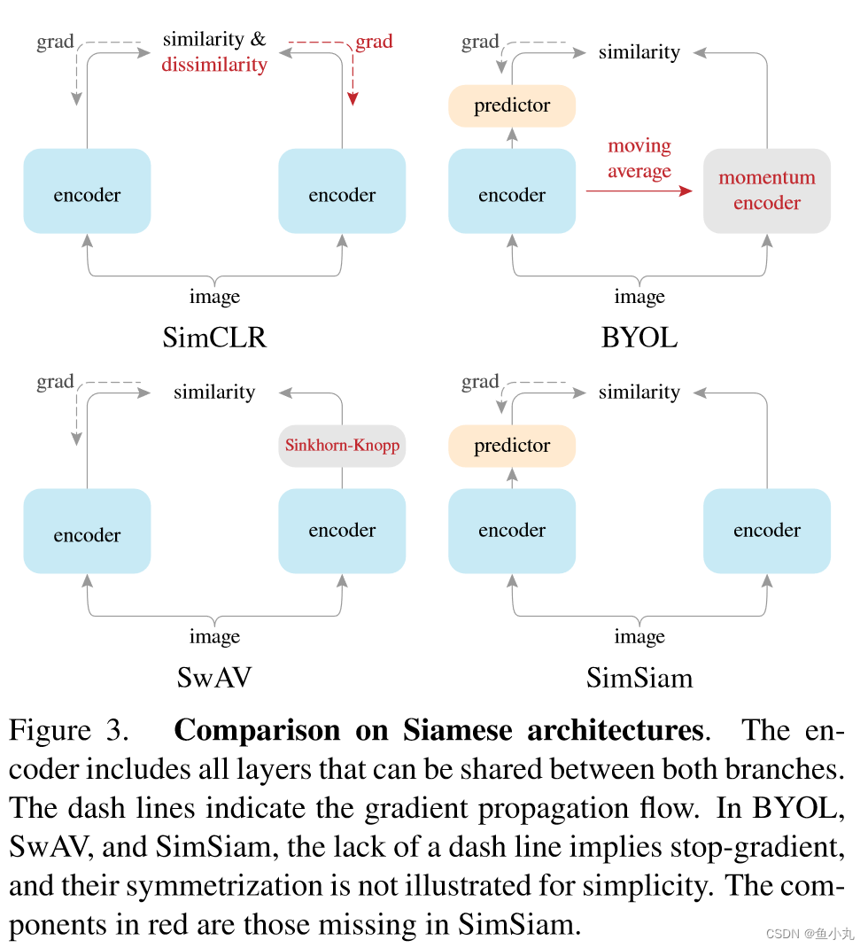
SimSiam
论文:https://arxiv.org/abs/2011.10566
代码:https://github.com/facebookresearch/simsiam
论文写的很好了,大家都去看论文吧。代码很简单和伪代码差不多。


 2751
2751


 被折叠的 条评论
为什么被折叠?
被折叠的 条评论
为什么被折叠?
 到【灌水乐园】发言


