


来自吴恩达深度学习系列视频:卷积神经网络第四周作业2: Art Generation with Neural Style Transfer - v1。如果英文阅读对你来说有障碍,可以参考【中英】【吴恩达课后编程作业】Course 4 -卷积神经网络 - 第四周作业。参照对代码的注释并不完全正确,该作业中有一个很难发现的错误,我在下面注明了。
预训练模型你可以在原论文官网 MatConvNet. http://www.vlfeat.org/matconvnet/pretrained/ 找到并下载。
完整的ipynb文件参见博主github: https://github.com/Hongze-Wang/Deep-Learning-Andrew-Ng/tree/master/homework
Deep Learning & Art: Neural Style Transfer
Welcome to the second assignment of this week. In this assignment, you will learn about Neural Style Transfer. This algorithm was created by Gatys et al. (2015) (https://arxiv.org/abs/1508.06576).
In this assignment, you will:
- Implement the neural style transfer algorithm
- Generate novel artistic images using your algorithm
Most of the algorithms you’ve studied optimize a cost function to get a set of parameter values. In Neural Style Transfer, you’ll optimize a cost function to get pixel values!
import os
import sys
import scipy.io
import scipy.misc
import matplotlib.pyplot as plt
from matplotlib.pyplot import imshow
from PIL import Image
from nst_utils import *
import numpy as np
import tensorflow as tf

%matplotlib inline
1 - Problem Statement
Neural Style Transfer (NST) is one of the most fun techniques in deep learning. As seen below, it merges two images, namely, a “content” image © and a “style” image (S), to create a “generated” image (G). The generated image G combines the “content” of the image C with the “style” of image S.
In this example, you are going to generate an image of the Louvre museum in Paris (content image C), mixed with a painting by Claude Monet, a leader of the impressionist movement (style image S).
Let’s see how you can do this.
2 - Transfer Learning
Neural Style Transfer (NST) uses a previously trained convolutional network, and builds on top of that. The idea of using a network trained on a different task and applying it to a new task is called transfer learning.
Following the original NST paper (https://arxiv.org/abs/1508.06576), we will use the VGG network. Specifically, we’ll use VGG-19, a 19-layer version of the VGG network. This model has already been trained on the very large ImageNet database, and thus has learned to recognize a variety of low level features (at the earlier layers) and high level features (at the deeper layers).
Run the following code to load parameters from the VGG model. This may take a few seconds.
model = load_vgg_model("pretrained-model/imagenet-vgg-verydeep-19.mat")
print(model)
{'input': <tf.Variable 'Variable:0' shape=(1, 300, 400, 3) dtype=float32_ref>, 'conv1_1': <tf.Tensor 'Relu:0' shape=(1, 300, 400, 64) dtype=float32>, 'conv1_2': <tf.Tensor 'Relu_1:0' shape=(1, 300, 400, 64) dtype=float32>, 'avgpool1': <tf.Tensor 'AvgPool:0' shape=(1, 150, 200, 64) dtype=float32>, 'conv2_1': <tf.Tensor 'Relu_2:0' shape=(1, 150, 200, 128) dtype=float32>, 'conv2_2': <tf.Tensor 'Relu_3:0' shape=(1, 150, 200, 128) dtype=float32>, 'avgpool2': <tf.Tensor 'AvgPool_1:0' shape=(1, 75, 100, 128) dtype=float32>, 'conv3_1': <tf.Tensor 'Relu_4:0' shape=(1, 75, 100, 256) dtype=float32>, 'conv3_2': <tf.Tensor 'Relu_5:0' shape=(1, 75, 100, 256) dtype=float32>, 'conv3_3': <tf.Tensor 'Relu_6:0' shape=(1, 75, 100, 256) dtype=float32>, 'conv3_4': <tf.Tensor 'Relu_7:0' shape=(1, 75, 100, 256) dtype=float32>, 'avgpool3': <tf.Tensor 'AvgPool_2:0' shape=(1, 38, 50, 256) dtype=float32>, 'conv4_1': <tf.Tensor 'Relu_8:0' shape=(1, 38, 50, 512) dtype=float32>, 'conv4_2': <tf.Tensor 'Relu_9:0' shape=(1, 38, 50, 512) dtype=float32>, 'conv4_3': <tf.Tensor 'Relu_10:0' shape=(1, 38, 50, 512) dtype=float32>, 'conv4_4': <tf.Tensor 'Relu_11:0' shape=(1, 38, 50, 512) dtype=float32>, 'avgpool4': <tf.Tensor 'AvgPool_3:0' shape=(1, 19, 25, 512) dtype=float32>, 'conv5_1': <tf.Tensor 'Relu_12:0' shape=(1, 19, 25, 512) dtype=float32>, 'conv5_2': <tf.Tensor 'Relu_13:0' shape=(1, 19, 25, 512) dtype=float32>, 'conv5_3': <tf.Tensor 'Relu_14:0' shape=(1, 19, 25, 512) dtype=float32>, 'conv5_4': <tf.Tensor 'Relu_15:0' shape=(1, 19, 25, 512) dtype=float32>, 'avgpool5': <tf.Tensor 'AvgPool_4:0' shape=(1, 10, 13, 512) dtype=float32>}
The model is stored in a python dictionary where each variable name is the key and the corresponding value is a tensor containing that variable’s value. To run an image through this network, you just have to feed the image to the model. In TensorFlow, you can do so using the tf.assign function. In particular, you will use the assign function like this:
model["input"].assign(image)
This assigns the image as an input to the model. After this, if you want to access the activations of a particular layer, say layer 4_2 when the network is run on this image, you would run a TensorFlow session on the correct tensor conv4_2, as follows:
sess.run(model["conv4_2"])
3 - Neural Style Transfer
We will build the NST algorithm in three steps:
- Build the content cost function Jcontent(C,G)J_{content}(C,G)Jcontent(C,G)
- Build the style cost function Jstyle(S,G)J_{style}(S,G)Jstyle(S,G)
- Put it together to get J(G)=αJcontent(C,G)+βJstyle(S,G)J(G) = \alpha J_{content}(C,G) + \beta J_{style}(S,G)J(G)=αJcontent(C,G)+βJstyle(S,G).
3.1 - Computing the content cost
In our running example, the content image C will be the picture of the Louvre Museum in Paris. Run the code below to see a picture of the Louvre.
content_image = scipy.misc.imread("images/louvre.jpg")
imshow(content_image)
C:\Users\wangh\Anaconda3\envs\tensorflow\lib\site-packages\ipykernel_launcher.py:1: DeprecationWarning: `imread` is deprecated!
`imread` is deprecated in SciPy 1.0.0, and will be removed in 1.2.0.
Use ``imageio.imread`` instead.
  """Entry point for launching an IPython kernel.
<matplotlib.image.AxesImage at 0x1a500056f60>
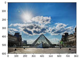
The content image © shows the Louvre museum’s pyramid surrounded by old Paris buildings, against a sunny sky with a few clouds.
** 3.1.1 - How do you ensure the generated image G matches the content of the image C?**
As we saw in lecture, the earlier (shallower) layers of a ConvNet tend to detect lower-level features such as edges and simple textures, and the later (deeper) layers tend to detect higher-level features such as more complex textures as well as object classes.
We would like the “generated” image G to have similar content as the input image C. Suppose you have chosen some layer’s activations to represent the content of an image. In practice, you’ll get the most visually pleasing results if you choose a layer in the middle of the network–neither too shallow nor too deep. (After you have finished this exercise, feel free to come back and experiment with using different layers, to see how the results vary.)
So, suppose you have picked one particular hidden layer to use. Now, set the image C as the input to the pretrained VGG network, and run forward propagation. Let a(C)a^{(C)}a(C) be the hidden layer activations in the layer you had chosen. (In lecture, we had written this as a[l](C)a^{[l](C)}a[l](C), but here we’ll drop the superscript [l][l][l] to simplify the notation.) This will be a nH×nW×nCn_H \times n_W \times n_CnH×nW×nCtensor. Repeat this process with the image G: Set G as the input, and run forward progation. Leta(G)a^{(G)}a(G)be the corresponding hidden layer activation. We will define as the content cost function as:
Jcontent(C,G)=14×nH×nW×nC∑all entries(a(C)−a(G))2(1)J_{content}(C,G) = \frac{1}{4 \times n_H \times n_W \times n_C}\sum _{ \text{all entries}} (a^{(C)} - a^{(G)})^2\tag{1}Jcontent(C,G)=4×nH×nW×nC1all entries∑(a(C)−a(G))2(1)
Here, nH,nWn_H, n_WnH,nW and nCn_CnC are the height, width and number of channels of the hidden layer you have chosen, and appear in a normalization term in the cost. For clarity, note that a(C)a^{(C)}a(C) and a(G)a^{(G)}a(G) are the volumes corresponding to a hidden layer’s activations. In order to compute the cost Jcontent(C,G)J_{content}(C,G)Jcontent(C,G), it might also be convenient to unroll these 3D volumes into a 2D matrix, as shown below. (Technically this unrolling step isn’t needed to compute JcontentJ_{content}Jcontent, but it will be good practice for when you do need to carry out a similar operation later for computing the style const JstyleJ_{style}Jstyle.)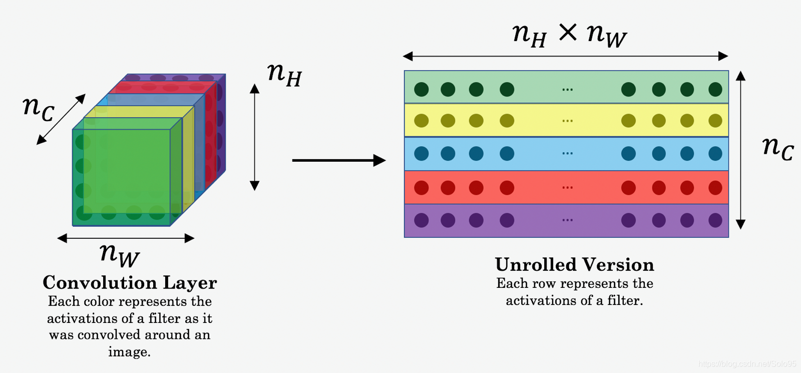
Exercise: Compute the “content cost” using TensorFlow.
Instructions: The 3 steps to implement this function are:
- Retrieve dimensions from a_G:
- To retrieve dimensions from a tensor X, use:
X.get_shape().as_list()
- To retrieve dimensions from a tensor X, use:
- Unroll a_C and a_G as explained in the picture above
- Compute the content cost:
# GRADED FUNCTION: compute_content_cost

def compute_content_cost(a_C, a_G):
    """
    Computes the content cost

    Arguments:
    a_C -- tensor of dimension (1, n_H, n_W, n_C), hidden layer activations representing content of the image C
    a_G -- tensor of dimension (1, n_H, n_W, n_C), hidden layer activations representing content of the image G

    Returns:
    J_content -- scalar that you compute using equation 1 above.
    """

    ### START CODE HERE ###
    # Retrieve dimensions from a_G (≈1 line)
    m, n_H, n_W, n_C = a_G.get_shape().as_list()

    # Reshape a_C and a_G (≈2 lines)
    a_C_unrolled = tf.reshape(a_C,shape=(n_H* n_W,n_C))
    a_G_unrolled = tf.reshape(a_G,shape=(n_H* n_W,n_C))

    # compute the cost with tensorflow (≈1 line)
    J_content = tf.reduce_sum(tf.square(tf.subtract(a_C_unrolled,a_G_unrolled)))/(4*n_H*n_W*n_C)
    ### END CODE HERE ###

    return J_content
tf.reset_default_graph()

with tf.Session() as test:
    tf.set_random_seed(1)
    a_C = tf.random_normal([1, 4, 4, 3], mean=1, stddev=4)
    a_G = tf.random_normal([1, 4, 4, 3], mean=1, stddev=4)
    J_content = compute_content_cost(a_C, a_G)
    print("J_content = " + str(J_content.eval()))
J_content = 6.7655926
3.2 - Computing the style cost
For our running example, we will use the following style image:
style_image = scipy.misc.imread("images/monet_800600.jpg")
imshow(style_image)
C:\Users\wangh\Anaconda3\envs\tensorflow\lib\site-packages\ipykernel_launcher.py:1: DeprecationWarning: `imread` is deprecated!
`imread` is deprecated in SciPy 1.0.0, and will be removed in 1.2.0.
Use ``imageio.imread`` instead.
  """Entry point for launching an IPython kernel.
<matplotlib.image.AxesImage at 0x1a5002ab048>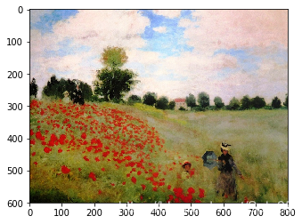
This painting was painted in the style of impressionism.
Lets see how you can now define a “style” const function Jstyle(S,G)J_{style}(S,G)Jstyle(S,G).
3.2.1 - Style matrix
The style matrix is also called a “Gram matrix.” In linear algebra, the Gram matrix G of a set of vectors (v1,…,vn)(v_{1},\dots ,v_{n})(v1,…,vn) is the matrix of dot products, whose entries are Gij=vTivj=np.dot(vi,vj){\displaystyle G_{ij} = v_{i}^T v_{j} = np.dot(v_{i}, v_{j}) }Gij=viTvj=np.dot(vi,vj). In other words, GijG_{ij}Gij compares how similar viv_ivi is to vjv_jvj: If they are highly similar, you would expect them to have a large dot product, and thus for GijG_{ij}Gij to be large.
Note that there is an unfortunate collision in the variable names used here. We are following common terminology used in the literature, but GGG is used to denote the Style matrix (or Gram matrix) as well as to denote the generated image GGG. We will try to make sure which GGGwe are referring to is always clear from the context.
In NST, you can compute the Style matrix by multiplying the “unrolled” filter matrix with their transpose: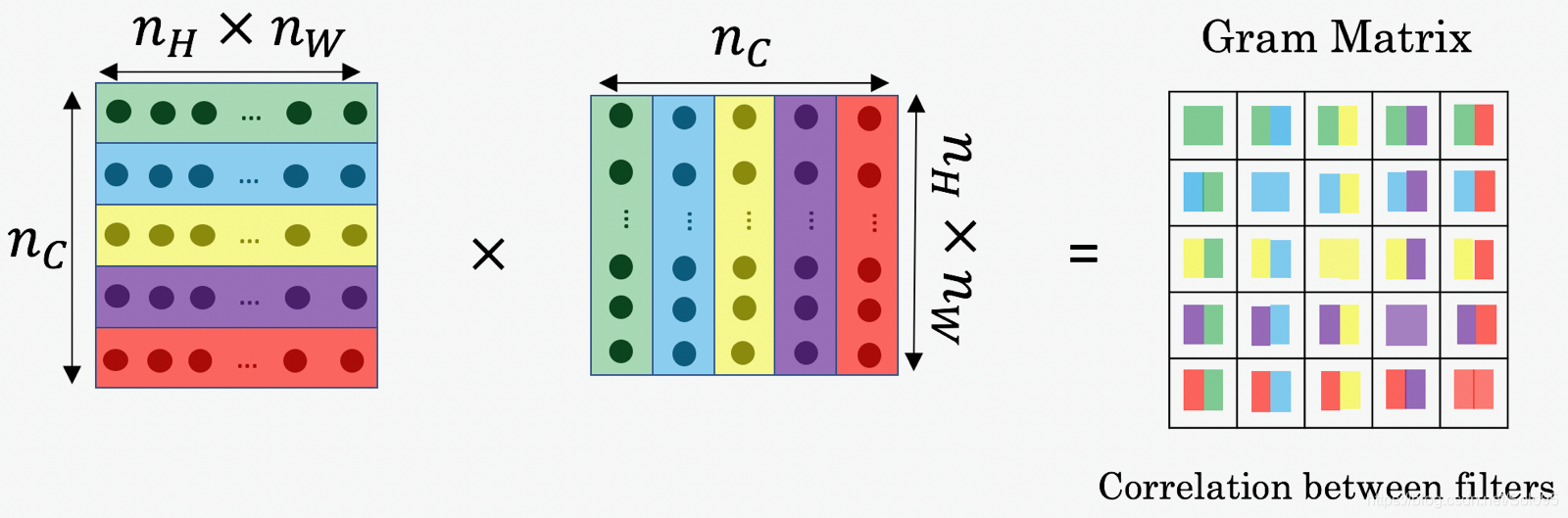
The result is a matrix of dimension (nC,nC)(n_C,n_C)(nC,nC) where nCn_CnC is the number of filters. The value GijG_{ij}Gijmeasures how similar the activations of filter iii are to the activations of filter jjj.
One important part of the gram matrix is that the diagonal elements such as GiiG_{ii}Gii also measures how active filter iii is. For example, suppose filter iii is detecting vertical textures in the image. Then GiiG_{ii}Gii measures how common vertical textures are in the image as a whole: If GiiG_{ii}Gii is large, this means that the image has a lot of vertical texture.
By capturing the prevalence of different types of features (GiiG_{ii}Gii), as well as how much different features occur together (GijG_{ij}Gij), the Style matrix GGG measures the style of an image.
Exercise:
Using TensorFlow, implement a function that computes the Gram matrix of a matrix A. The formula is: The gram matrix of A is GA=AATG_A = AA^TGA=AAT. If you are stuck, take a look at Hint 1 and Hint 2.
# GRADED FUNCTION: gram_matrix

def gram_matrix(A):
    """
    Argument:
    A -- matrix of shape (n_C, n_H*n_W)

    Returns:
    GA -- Gram matrix of A, of shape (n_C, n_C)
    """

    ### START CODE HERE ### (≈1 line)
    GA = tf.matmul(A, tf.transpose(A)) # GA = tf.matmul(A, A, transpose_b = True)
    ### END CODE HERE ###

    return GA
tf.reset_default_graph()

with tf.Session() as test:
    tf.set_random_seed(1)
    A = tf.random_normal([3, 2*1], mean=1, stddev=4)
    GA = gram_matrix(A)

    print("GA = " + str(GA.eval()))
GA = [[ 6.422305 -4.429122 -2.096682]
 [-4.429122 19.465837 19.563871]
 [-2.096682 19.563871 20.686462]]
3.2.2 - Style cost
After generating the Style matrix (Gram matrix), your goal will be to minimize the distance between the Gram matrix of the “style” image S and that of the “generated” image G. For now, we are using only a single hidden layer a[l]a^{[l]}a[l], and the corresponding style cost for this layer is defined as:
J[l]style(S,G)=14×nC2×(nH×nW)2∑nCi=1∑nCj=1(G(S)ij−G(G)ij)2(2)J_{style}^{[l]}(S,G) = \frac{1}{4 \times {n_C}^2 \times (n_H \times n_W)^2} \sum _{i=1}^{n_C}\sum_{j=1}^{n_C}(G^{(S)}_{ij} - G^{(G)}_{ij})^2\tag{2}Jstyle[l](S,G)=4×nC2×(nH×nW)21i=1∑nCj=1∑nC(Gij(S)−Gij(G))2(2)
where G(S)G^{(S)}G(S) and G(G)G^{(G)}G(G) are respectively the Gram matrices of the “style” image and the “generated” image, computed using the hidden layer activations for a particular hidden layer in the network.
Exercise: Compute the style cost for a single layer.
Instructions: The 3 steps to implement this function are:
- Retrieve dimensions from the hidden layer activations a_G:
- To retrieve dimensions from a tensor X, use:
X.get_shape().as_list()
- To retrieve dimensions from a tensor X, use:
- Unroll the hidden layer activations a_S and a_G into 2D matrices, as explained in the picture above.
- Compute the Style matrix of the images S and G. (Use the function you had previously written.)
- Compute the Style cost:
# GRADED FUNCTION: compute_layer_style_cost

def compute_layer_style_cost(a_S, a_G):
    """
    Arguments:
    a_S -- tensor of dimension (1, n_H, n_W, n_C), hidden layer activations representing style of the image S
    a_G -- tensor of dimension (1, n_H, n_W, n_C), hidden layer activations representing style of the image G

    Returns:
    J_style_layer -- tensor representing a scalar value, style cost defined above by equation (2)
    """

    ### START CODE HERE ###
    # Retrieve dimensions from a_G (≈1 line)
    m, n_H, n_W, n_C = a_G.get_shape().as_list()

    # Reshape the images to have them of shape (n_H*n_W, n_C) (≈2 lines)
    a_S = tf.transpose(tf.reshape(a_S, [n_H*n_W, n_C]))
    a_G = tf.transpose(tf.reshape(a_G, [n_H*n_W, n_C]))

    # Computing gram_matrices for both images S and G (≈2 lines)
    GS = gram_matrix(a_S)
    GG = gram_matrix(a_G)

    # Computing the loss (≈1 line)
    J_style_layer = tf.reduce_sum(tf.square(tf.subtract(GS, GG))) / (4 * n_C * n_C * n_H * n_W * n_H * n_W )
    # Do not use np.square(n_C) you can pass the following test but can't use in the CNN

    ### END CODE HERE ###

    return J_style_layer
tf.reset_default_graph()

with tf.Session() as test:
    tf.set_random_seed(1)
    a_S = tf.random_normal([1, 4, 4, 3], mean=1, stddev=4)
    a_G = tf.random_normal([1, 4, 4, 3], mean=1, stddev=4)
    J_style_layer = compute_layer_style_cost(a_S, a_G)

    print("J_style_layer = " + str(J_style_layer.eval()))
J_style_layer = 9.190278
3.2.3 Style Weights
So far you have captured the style from only one layer. We’ll get better results if we “merge” style costs from several different layers. After completing this exercise, feel free to come back and experiment with different weights to see how it changes the generated image GGG. But for now, this is a pretty reasonable default:
STYLE_LAYERS = [
    ('conv1_1', 0.2),
    ('conv2_1', 0.2),
    ('conv3_1', 0.2),
    ('conv4_1', 0.2),
    ('conv5_1', 0.2)]
You can combine the style costs for different layers as follows:
Jstyle(S,G)=∑lλ[l]J[l]style(S,G)J_{style}(S,G) = \sum_{l} \lambda^{[l]} J^{[l]}_{style}(S,G)Jstyle(S,G)=l∑λ[l]Jstyle[l](S,G)
where the values for λ[l]\lambda^{[l]}λ[l] are given in STYLE_LAYERS.
We’ve implemented a compute_style_cost(…) function. It simply calls your compute_layer_style_cost(...) several times, and weights their results using the values in STYLE_LAYERS. Read over it to make sure you understand what it’s doing.
def compute_style_cost(model, STYLE_LAYERS):
    """
    Computes the overall style cost from several chosen layers

    Arguments:
    model -- our tensorflow model
    STYLE_LAYERS -- A python list containing:
                        - the names of the layers we would like to extract style from
                        - a coefficient for each of them

    Returns:
    J_style -- tensor representing a scalar value, style cost defined above by equation (2)
    """

    # initialize the overall style cost
    J_style = 0

    for layer_name, coeff in STYLE_LAYERS:

        # Select the output tensor of the currently selected layer
        out = model[layer_name]

        # Set a_S to be the hidden layer activation from the layer we have selected, by running the session on out
        a_S = sess.run(out)

        # Set a_G to be the hidden layer activation from same layer. Here, a_G references model[layer_name]
        # and isn't evaluated yet. Later in the code, we'll assign the image G as the model input, so that
        # when we run the session, this will be the activations drawn from the appropriate layer, with G as input.
        a_G = out

        # Compute style_cost for the current layer
        J_style_layer = compute_layer_style_cost(a_S, a_G)

        # Add coeff * J_style_layer of this layer to overall style cost
        J_style += coeff * J_style_layer

    return J_style
Note: In the inner-loop of the for-loop above, a_G is a tensor and hasn’t been evaluated yet. It will be evaluated and updated at each iteration when we run the TensorFlow graph in model_nn() below.
3.3 - Defining the total cost to optimize
Finally, let’s create a cost function that minimizes both the style and the content cost. The formula is:
J(G)=αJcontent(C,G)+βJstyle(S,G)J(G) = \alpha J_{content}(C,G) + \beta J_{style}(S,G)J(G)=αJcontent(C,G)+βJstyle(S,G)
Exercise: Implement the total cost function which includes both the content cost and the style cost.
# GRADED FUNCTION: total_cost

def total_cost(J_content, J_style, alpha = 10, beta = 40):
    """
    Computes the total cost function

    Arguments:
    J_content -- content cost coded above
    J_style -- style cost coded above
    alpha -- hyperparameter weighting the importance of the content cost
    beta -- hyperparameter weighting the importance of the style cost

    Returns:
    J -- total cost as defined by the formula above.
    """

    ### START CODE HERE ### (≈1 line)
    J = alpha * J_content + beta * J_style
    ### END CODE HERE ###

    return J
tf.reset_default_graph()

with tf.Session() as test:
    np.random.seed(3)
    J_content = np.random.randn()
    J_style = np.random.randn()
    J = total_cost(J_content, J_style)
    print("J = " + str(J))
J = 35.34667875478276
4 - Solving the optimization problem
Finally, let’s put everything together to implement Neural Style Transfer!
Here’s what the program will have to do:
1. Create an Interactive Session 2. Load the content image 3. Load the style image 4. Randomly initialize the image to be generated 5. Load the VGG16 model 7. Build the TensorFlow graph: - Run the content image through the VGG16 model and compute the content cost - Run the style image through the VGG16 model and compute the style cost - Compute the total cost - Define the optimizer and the learning rate 8. Initialize the TensorFlow graph and run it for a large number of iterations, updating the generated image at every step. Lets go through the individual steps in detail.
You’ve previously implemented the overall cost J(G)J(G)J(G). We’ll now set up TensorFlow to optimize this with respect to GGG. To do so, your program has to reset the graph and use an “Interactive Session”. Unlike a regular session, the “Interactive Session” installs itself as the default session to build a graph. This allows you to run variables without constantly needing to refer to the session object, which simplifies the code.
Lets start the interactive session.
# Reset the graph
tf.reset_default_graph()

# Start interactive session
sess = tf.InteractiveSession()
Let’s load, reshape, and normalize our “content” image (the Louvre museum picture):
content_image = scipy.misc.imread("images/louvre_small.jpg")
content_image = reshape_and_normalize_image(content_image)
C:\Users\wangh\Anaconda3\envs\tensorflow\lib\site-packages\ipykernel_launcher.py:1: DeprecationWarning: `imread` is deprecated!
`imread` is deprecated in SciPy 1.0.0, and will be removed in 1.2.0.
Use ``imageio.imread`` instead.
  """Entry point for launching an IPython kernel.
Let’s load, reshape and normalize our “style” image (Claude Monet’s painting):
style_image = scipy.misc.imread("images/monet.jpg")
style_image = reshape_and_normalize_image(style_image)
C:\Users\wangh\Anaconda3\envs\tensorflow\lib\site-packages\ipykernel_launcher.py:1: DeprecationWarning: `imread` is deprecated!
`imread` is deprecated in SciPy 1.0.0, and will be removed in 1.2.0.
Use ``imageio.imread`` instead.
  """Entry point for launching an IPython kernel.
Now, we initialize the “generated” image as a noisy image created from the content_image. By initializing the pixels of the generated image to be mostly noise but still slightly correlated with the content image, this will help the content of the “generated” image more rapidly match the content of the “content” image. (Feel free to look in nst_utils.py to see the details of generate_noise_image(...); to do so, click “File–>Open…” at the upper-left corner of this Jupyter notebook.)
generated_image = generate_noise_image(content_image)
imshow(generated_image[0])
Clipping input data to the valid range for imshow with RGB data ([0..1] for floats or [0..255] for integers).
<matplotlib.image.AxesImage at 0x1a502693eb8>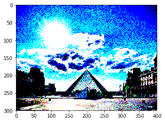
Next, as explained in part (2), let’s load the VGG16 model.
model = load_vgg_model("pretrained-model/imagenet-vgg-verydeep-19.mat")
To get the program to compute the content cost, we will now assign a_C and a_G to be the appropriate hidden layer activations. We will use layer conv4_2 to compute the content cost. The code below does the following:
- Assign the content image to be the input to the VGG model.
- Set a_C to be the tensor giving the hidden layer activation for layer “conv4_2”.
- Set a_G to be the tensor giving the hidden layer activation for the same layer.
- Compute the content cost using a_C and a_G.
# Assign the content image to be the input of the VGG model.
sess.run(model['input'].assign(content_image))

# Select the output tensor of layer conv4_2
out = model['conv4_2']

# Set a_C to be the hidden layer activation from the layer we have selected
a_C = sess.run(out)

# Set a_G to be the hidden layer activation from same layer. Here, a_G references model['conv4_2']
# and isn't evaluated yet. Later in the code, we'll assign the image G as the model input, so that
# when we run the session, this will be the activations drawn from the appropriate layer, with G as input.
a_G = out

# Compute the content cost
J_content = compute_content_cost(a_C, a_G)
Note: At this point, a_G is a tensor and hasn’t been evaluated. It will be evaluated and updated at each iteration when we run the Tensorflow graph in model_nn() below.
# Assign the input of the model to be the "style" image
sess.run(model['input'].assign(style_image))

# Compute the style cost
J_style = compute_style_cost(model, STYLE_LAYERS)
Exercise: Now that you have J_content and J_style, compute the total cost J by calling total_cost(). Use alpha = 10 and beta = 40.
### START CODE HERE ### (1 line)
J = total_cost(J_content, J_style, alpha=10, beta=40)
### END CODE HERE ###
You’d previously learned how to set up the Adam optimizer in TensorFlow. Lets do that here, using a learning rate of 2.0. See reference
# define optimizer (1 line)
optimizer = tf.train.AdamOptimizer(2.0)

# define train_step (1 line)
train_step = optimizer.minimize(J)
Exercise: Implement the model_nn() function which initializes the variables of the tensorflow graph, assigns the input image (initial generated image) as the input of the VGG16 model and runs the train_step for a large number of steps.
def model_nn(sess, input_image, num_iterations = 200):

    # Initialize global variables (you need to run the session on the initializer)
    ### START CODE HERE ### (1 line)
    sess.run(tf.global_variables_initializer())
    ### END CODE HERE ###

    # Run the noisy input image (initial generated image) through the model. Use assign().
    ### START CODE HERE ### (1 line)
    generated_image=sess.run(model['input'].assign(input_image))
    ### END CODE HERE ###

    for i in range(num_iterations):

        # Run the session on the train_step to minimize the total cost
        ### START CODE HERE ### (1 line)
        sess.run(train_step)
        ### END CODE HERE ###

        # Compute the generated image by running the session on the current model['input']
        ### START CODE HERE ### (1 line)
        generated_image = sess.run(model['input'])
        ### END CODE HERE ###

        # Print every 20 iteration.
        if i%20 == 0:
            Jt, Jc, Js = sess.run([J, J_content, J_style])
            print("Iteration " + str(i) + " :")
            print("total cost = " + str(Jt))
            print("content cost = " + str(Jc))
            print("style cost = " + str(Js))

            # save current generated image in the "/output" directory
            save_image("output/" + str(i) + ".png", generated_image)

    # save last generated image
    save_image('output/generated_image.jpg', generated_image)

    return generated_image
Run the following cell to generate an artistic image. It should take about 3min on CPU for every 20 iterations but you start observing attractive results after ≈140 iterations. Neural Style Transfer is generally trained using GPUs.
<span style="color:#000000"><code class="language-python">model_nn<span style="color:#999999">(</span>sess<span style="color:#999999">,</span> generated_image<span style="color:#999999">)</span>
</code></span>- 1
我们的结果可能与作业中给出的答案有一点差距,是由于tensoflow版本的差别导致的,只要你跟我的结果一样,就说明你的代码没有错误。
Iteration 0 :
total cost = 4934349000.0
content cost = 7861.214
style cost = 123356750.0
Iteration 20 :
total cost = 932611600.0
content cost = 15132.663
style cost = 23311508.0
Iteration 40 :
total cost = 477627420.0
content cost = 16783.37
style cost = 11936490.0
Iteration 60 :
total cost = 306697860.0
content cost = 17380.822
style cost = 7663101.0
Iteration 80 :
total cost = 223841800.0
content cost = 17668.08
style cost = 5591627.5
Iteration 100 :
total cost = 176972400.0
content cost = 17870.701
style cost = 4419842.5
Iteration 120 :
total cost = 146694260.0
content cost = 18021.35
style cost = 3662851.2
Iteration 140 :
total cost = 125131070.0
content cost = 18153.928
style cost = 3123738.5
Iteration 160 :
total cost = 108790870.0
content cost = 18272.299
style cost = 2715203.8
Iteration 180 :
total cost = 95894750.0
content cost = 18393.818
style cost = 2392770.5
array([[[[ -49.67133  ,  -58.251316 ,   48.095398 ],
         [ -25.372385 ,  -38.168175 ,   37.27234  ],
         [ -43.016766 ,  -27.774094 ,   15.616587 ],
         ...,
         [ -24.851778 ,  -11.482686 ,   14.043713 ],
         [ -28.261759 ,   -5.432111 ,   22.892218 ],
         [ -37.730164 ,   -4.4746313,   51.073856 ]],

        [[ -63.22666  ,  -48.98665  ,   32.1745   ],
         [ -32.38033  ,  -29.24593  ,    2.3130383],
         [ -28.153406 ,  -30.149511 ,   16.600147 ],
         ...,
         [ -25.91221  ,   -9.283931 ,   24.660099 ],
         [ -19.217525 ,  -18.626879 ,   13.115261 ],
         [ -35.882973 ,   -7.36522  ,   10.447336 ]],

        [[ -53.831898 ,  -49.563393 ,   16.395382 ],
         [ -37.250004 ,  -40.06393  ,   -3.4430506],
         [ -35.500504 ,  -24.985638 ,    7.4599504],
         ...,
         [ -13.419331 ,  -40.166973 ,    9.971984 ],
         [ -14.162411 ,  -23.142082 ,   14.858548 ],
         [ -23.296358 ,  -19.798826 ,   13.086463 ]],

        ...,

        [[ -50.572655 ,  -46.64244  ,  -20.149261 ],
         [ -99.354095 ,  -74.578445 , -260.1668   ],
         [ -77.48133  ,  -72.94745  , -136.40567  ],
         ...,
         [ -68.834526 ,  -74.01386  ,  -34.98827  ],
         [ -83.054955 ,  -98.60898  ,  -28.64623  ],
         [  -1.2930164,  -30.425447 ,   21.960754 ]],

        [[ -33.281155 ,  -79.243416 ,   15.05997  ],
         [-189.83856  , -104.441    ,  -25.097038 ],
         [  14.234048 ,  -66.72137  ,   -8.623041 ],
         ...,
         [ -98.17861  ,  -89.279945 ,  -53.93503  ],
         [-108.455444 , -112.48683  ,  -67.32902  ],
         [ -68.08705  ,  -96.81742  ,   -1.4247434]],

        [[  36.238792 ,  -50.084637 ,   48.496128 ],
         [  23.921942 ,  -95.63244  ,   27.005836 ],
         [  33.516636 ,  -31.28835  ,   27.135208 ],
         ...,
         [-126.661804 , -106.955894 ,  -28.771286 ],
         [-161.2223   , -150.69933  ,  -45.33805  ],
         [ -27.795086 , -106.99931  ,   20.499334 ]]]], dtype=float32)
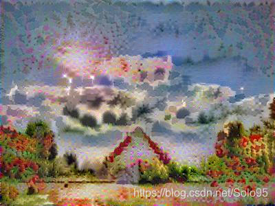
You’re done! After running this, in the upper bar of the notebook click on “File” and then “Open”. Go to the “/output” directory to see all the saved images. Open “generated_image” to see the generated image! ?
You should see something the image presented below on the right: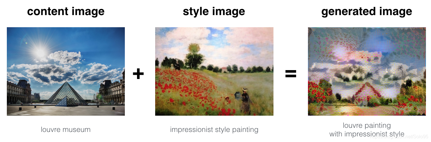 We didn’t want you to wait too long to see an initial result, and so had set the hyperparameters accordingly. To get the best looking results, running the optimization algorithm longer (and perhaps with a smaller learning rate) might work better. After completing and submitting this assignment, we encourage you to come back and play more with this notebook, and see if you can generate even better looking images.
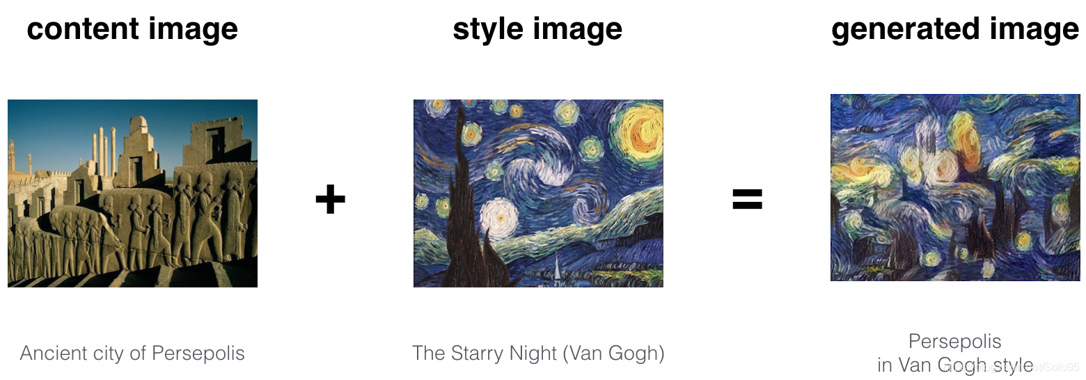
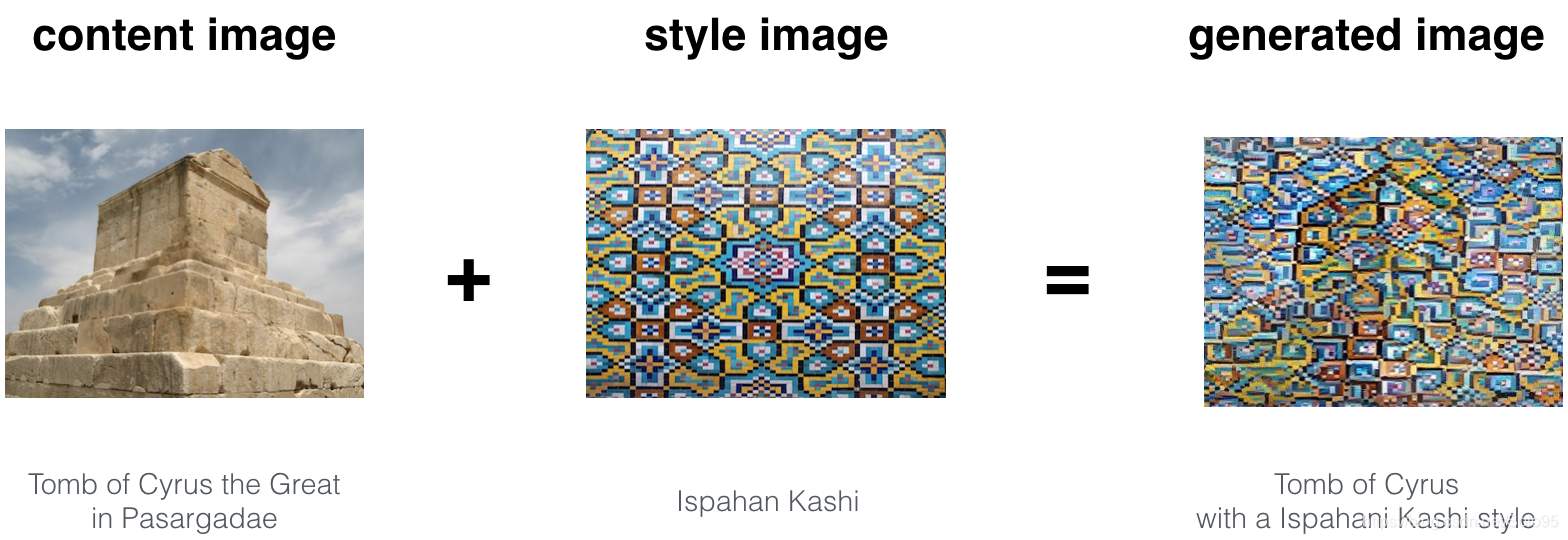
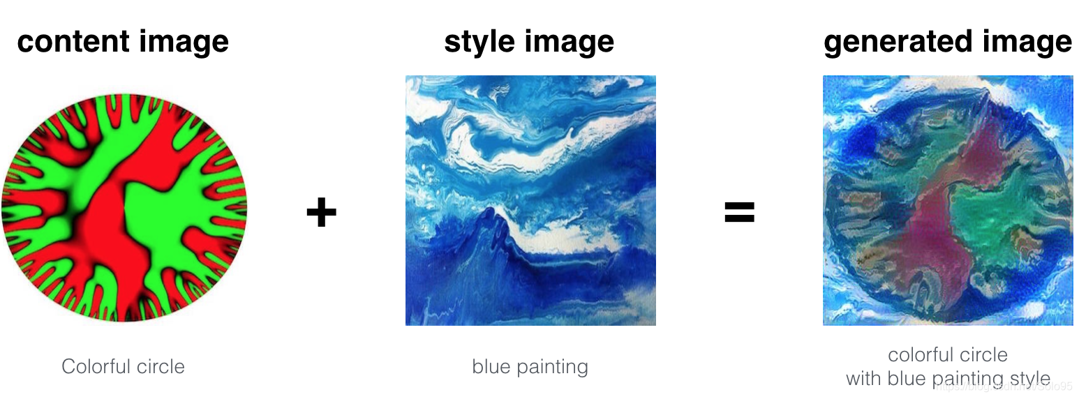
Here are few other examples:
-
The beautiful ruins of the ancient city of Persepolis (Iran) with the style of Van Gogh (The Starry Night)
-
The tomb of Cyrus the great in Pasargadae with the style of a Ceramic Kashi from Ispahan.
-
A scientific study of a turbulent fluid with the style of a abstract blue fluid painting.
5 - Test with your own image (Optional/Ungraded)
Finally, you can also rerun the algorithm on your own images!
To do so, go back to part 4 and change the content image and style image with your own pictures. In detail, here’s what you should do:
- Click on “File -> Open” in the upper tab of the notebook
- Go to “/images” and upload your images (requirement: (WIDTH = 300, HEIGHT = 225)), rename them “my_content.png” and “my_style.png” for example.
- Change the code in part (3.4) from :
content_image = scipy.misc.imread("images/louvre.jpg")
style_image = scipy.misc.imread("images/claude-monet.jpg")
content_image = scipy.misc.imread("images/my_content.jpg")
style_image = scipy.misc.imread("images/my_style.jpg")
- Rerun the cells (you may need to restart the Kernel in the upper tab of the notebook).
You can also tune your hyperparameters:
- Which layers are responsible for representing the style? STYLE_LAYERS
- How many iterations do you want to run the algorithm? num_iterations
- What is the relative weighting between content and style? alpha/beta
6 - Conclusion
Great job on completing this assignment! You are now able to use Neural Style Transfer to generate artistic images. This is also your first time building a model in which the optimization algorithm updates the pixel values rather than the neural network’s parameters. Deep learning has many different types of models and this is only one of them!
What you should remember: - Neural Style Transfer is an algorithm that given a content image C and a style image S can generate an artistic image - It uses representations (hidden layer activations) based on a pretrained ConvNet. - The content cost function is computed using one hidden layer's activations. - The style cost function for one layer is computed using the Gram matrix of that layer's activations. The overall style cost function is obtained using several hidden layers. - Optimizing the total cost function results in synthesizing new images.This was the final programming exercise of this course. Congratulations–you’ve finished all the programming exercises of this course on Convolutional Networks! We hope to also see you in Course 5, on Sequence models!
References:
The Neural Style Transfer algorithm was due to Gatys et al. (2015). Harish Narayanan and Github user “log0” also have highly readable write-ups from which we drew inspiration. The pre-trained network used in this implementation is a VGG network, which is due to Simonyan and Zisserman (2015). Pre-trained weights were from the work of the MathConvNet team.
- Leon A. Gatys, Alexander S. Ecker, Matthias Bethge, (2015). A Neural Algorithm of Artistic Style (https://arxiv.org/abs/1508.06576)
- Harish Narayanan, Convolutional neural networks for artistic style transfer. https://harishnarayanan.org/writing/artistic-style-transfer/
- Log0, TensorFlow Implementation of “A Neural Algorithm of Artistic Style”. http://www.chioka.in/tensorflow-implementation-neural-algorithm-of-artistic-style
- Karen Simonyan and Andrew Zisserman (2015). Very deep convolutional networks for large-scale image recognition (https://arxiv.org/pdf/1409.1556.pdf)
- MatConvNet. http://www.vlfeat.org/matconvnet/pretrained/


 269
269


 被折叠的 条评论
为什么被折叠?
被折叠的 条评论
为什么被折叠?
 到【灌水乐园】发言


