k-近邻算法用于实际应用

摘要：

本章所有内容数据均来自《机器学习实战》的数据，是对K近邻算法的应用以及熟练

实例1改进约会网站的配对效果

 题目描述：海伦喜欢在在线约会网站寻找适合自己的对象，但是她不是喜欢每一个人。她发现交往过三种类型的人：

  1.不喜欢的人

  2.魅力一般的人

  3.极具魅力的人

所以需要对网站的对象归入恰当的分类。她周一到周五喜欢魅力一般的人，而周末则更喜欢极具魅力的人。所以需要根据数据来分类

准备数据：

  数据在文本datingTestSet.txt中，每个样本占据一行，总共1000行，每个样本有3个特征：

   每年获得的飞行常客里程数

  玩视频游戏所消耗的时间

  每周消费的冰淇淋的公升

那么这些数据从文本读取后需要改写成分类器可以接受的格式。输出为样本矩阵和类标签向量

def file2matrix(filename):
	fr = open(filename)
	arrayOlines = fr.readlines()
	numberOfLines = len(arrayOlines)
	returnMat = zeros((numberOfLines,3))
	classLabelVector=[]
	index = 0
	for line in arrayOLines:
		line = line.strip()  #去回车
		listFromLine = line.split('\t')  #以\t分割
		returnMat[index,:] = listFromLine[0:3]
		classLabelVector.append(int(listFromLine[-1]))
		index+=1
	return returnMat,classLabelVector

其实python处理文本文件很容易。

reload(kNN)

datingDataMat,datingLabels =  kNN.file2matrix('datingTestSet2.txt')

>>> datingDataMat
array([[  4.09200000e+04,   8.32697600e+00,   9.53952000e-01],
       [  1.44880000e+04,   7.15346900e+00,   1.67390400e+00],
       [  2.60520000e+04,   1.44187100e+00,   8.05124000e-01],
       ..., 
       [  2.65750000e+04,   1.06501020e+01,   8.66627000e-01],
       [  4.81110000e+04,   9.13452800e+00,   7.28045000e-01],
       [  4.37570000e+04,   7.88260100e+00,   1.33244600e+00]])

接下来需要分析数据，使用Matplotlib创建散点图

>>> import matplotlib.pyplot as plt
>>> fig = plt.figure()
>>> ax = fig.add_subplot(111)
>>> ax.scatter(datingDataMat[:,1],datingDataMat[:,2]) #颜色以及尺寸标识了数据点属性类别

散点图使用datingDataMat矩阵的第二，第三列数据代表玩视频游戏所耗时间百分比，每周所消耗的冰淇凌公升数

由于没有样本分类的特征值。很难看到任何有用的数据模型信息。一般用采用色彩或其他记号标记不同分类

而展现的数据图如下：

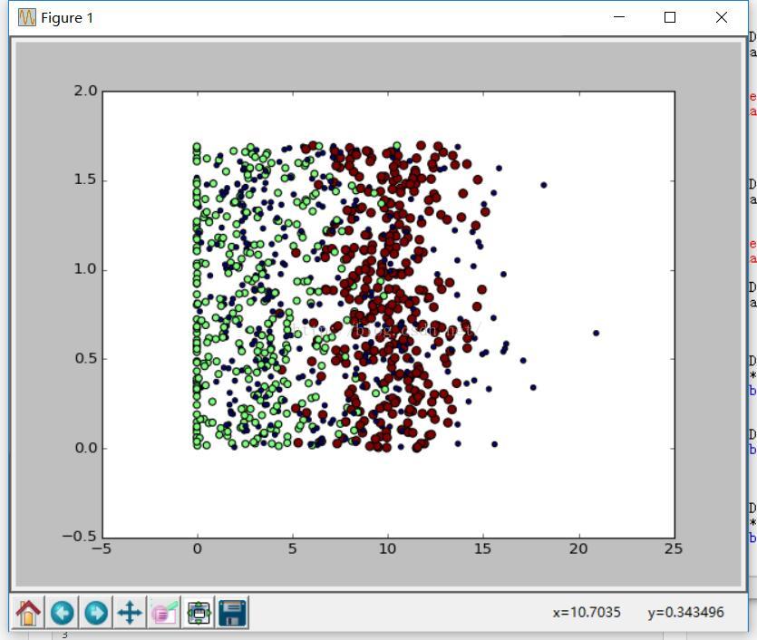
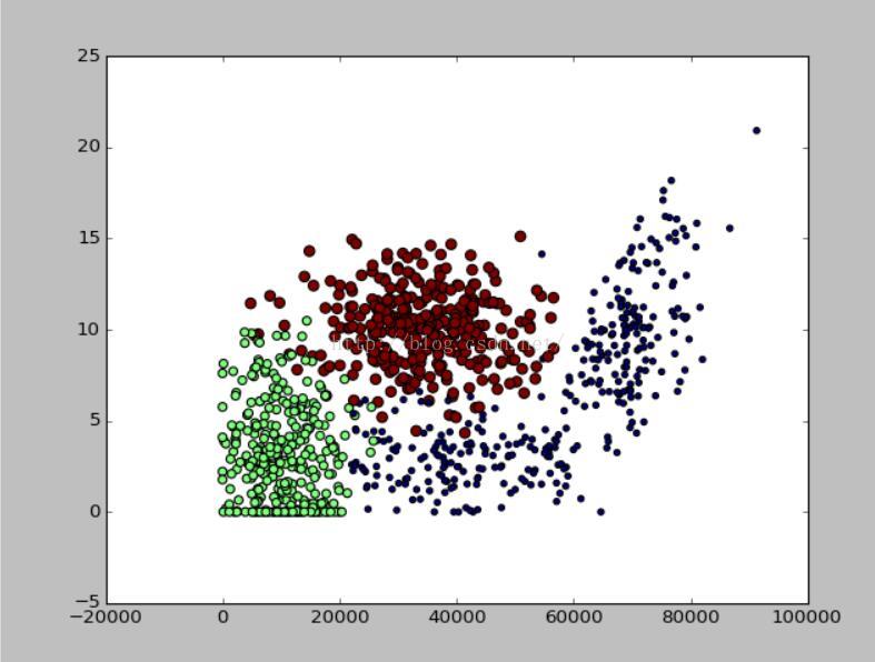
但是如果标识了三个不同的样本分类区域，采用第1.2列效果会更直观

对数据进行归一化处理：

如果我们对数据样本直接进行计算距离。(0-67)^2 + (20000-32000)^2 + (1.1-0.1)^2数字最大属性对结果影响很大。

也就是说飞行常客对于结果的影响远远大于其他特征。但是我们应该认为这3个属性同等重要。所i有需要数值归一化我们可以将任意值转化到

0到1之间  newValue = (oldValue-min)/(max-min)

def autoNorm(dataSet):
	minVals = dataSet.min(0)
	maxVals = dataSet.max(0)
	ranges = maxVals - minVals
	normDataSet = zeros(shape(dataSet))
	m = dataSet.shape[0]
	normDataSet = dataSet - tile(minVals,(m,1))
	normDataSet = normDataSet/tile(ranges,(m,1))
	return normDataSet,ranges,minVals

原来的数据为

array([[  4.09200000e+04,   8.32697600e+00,   9.53952000e-01],
       [  1.44880000e+04,   7.15346900e+00,   1.67390400e+00],
       [  2.60520000e+04,   1.44187100e+00,   8.05124000e-01],
       ..., 
       [  2.65750000e+04,   1.06501020e+01,   8.66627000e-01],
       [  4.81110000e+04,   9.13452800e+00,   7.28045000e-01],
       [  4.37570000e+04,   7.88260100e+00,   1.33244600e+00]])

进过处理后的数据为

array([[ 0.44832535,  0.39805139,  0.56233353],
       [ 0.15873259,  0.34195467,  0.98724416],
       [ 0.28542943,  0.06892523,  0.47449629],
       ..., 
       [ 0.29115949,  0.50910294,  0.51079493],
       [ 0.52711097,  0.43665451,  0.4290048 ],
       [ 0.47940793,  0.3768091 ,  0.78571804]])

测试算法：使用完成程序测试分类

机器学习的重要工作就是评估算法的正确率，通常按照上述的算法如果正确分类，那么可以使用这个软件来处理约会网站提供的约会名单了。

但是还需要测试当前分类器的性能，我们以测试错误率为主对这个程序测试程序如下：

def datingClassTest():
	hoRation = 0.10
	datingDataMat,datingLabels = file2matrix('E:\pythonProject\ML\datingTestSet2.txt')
	normMat,ranges,minVals = autoNorm(datingDataMat)
	m = normMat.shape[0]
	numTestVecs = int(m*hoRation)
	errorCount = 0.0
	for i in range(numTestVecs):
		classifierResult = classify0(normMat[i,:],normMat[numTestVecs:m,:],datingLabels[numTestVecs:m],3)
		print ("the classifier came back with %d,the real answer is %d"
		       %(classifierResult,datingLabels[i]))
		if(classifierResult!=datingLabels[i]):errorCount+=1.0
	print "the total error rate is %f" % (errorCount/float(numTestVecs))

其实就是计算错误个数占据总数的百分比，而最先给定的比率是测试集的个数

最后：进行泛化预测构造完整系统

上面已经对数据处理测试以及处理了，那么下面就是队数据进行预测

def classifyPerson():
	resultList = ['not at all','in small doses','in large doses']
	percentTats = float(raw_input("percentage of time spent playing?"))
	ffMiles = float(raw_input("frequent flier miles earned per year?"))
	iceCream = float(raw_input("liters of ice cream consume?"))
	datingDataMat,datingLabels = file2matrix('E:\pythonProject\ML\datingTestSet2.txt')
	normMat,ranges,minVals = autoNorm(datingDataMat)
	inArr = array([ffMiles,percentTats,iceCream])
	classifierResult = classify0((inArr-minVals)/ranges,normMat,datingLabels,3)
	print "You will probably like this person:",resultList[classifierResult-1]

根据类型输出喜好的程度

>>> kNN.classifyPerson()
percentage of time spent playing?10
frequent flier miles earned per year?10000
liters of ice cream consume?0.
You will probably like this person: in small doses