


一、首先先给出图示,什么叫卷积。(http://deeplearning.stanford.edu/wiki/index.php/)
当然很多人会疑问,为什么卷积后的图像会缩小,那是因为在进行图像滤波的时候边缘没有加0进行填充。正常的图像滤波边缘是会填充0,这样滤波出来的图像与原图像的大小保持一致。卷积可以用如下表示式来表示:
训练卷积核的方式(第一种):
当你在监督学习的时候你不用改变它的参数,它的参数时固定的。例如:你想提取人脸的特征,目前你已经有了自己的数据集,想训练9×9的卷积核(滤波器),这时你可以从你的数据集上取任意去9×9的小块,当然你取的小块越多,训练出来的卷积核越鲁棒。下面我按步骤来说明:
(1)取数据集上大量的小块,为训练滤波器做准备,滤波器的大小决定了你取小块的大小。
(2)如果你想得到20张特征图(这里的特征图是指不同的滤波器滤波后的结果图),那么你就需要20种不同的滤波器。那么如何得到这20种滤波器呢,这时你可以采用autoencoder学习,你的输入层为9×9=81个神经元,隐含层为20个神经元(隐含层的神经元个数决定了你滤波器的个数),输出层也为9×9=81个神经元,相当于一个自学习层,也称自监督学习。可以这样表示:输入→编码→解码→输出。这样经过参数学习后,就可以得到输入层到隐含层的参数,隐含层的每个神经元与输入层的81个神经元相连接,每个连接上是有参数的,一共含有81个参数,把81个参数reshape成9×9的参数,这样就得到1个滤波器,20个隐含层神经元分别与输入层81个神经元连接,这样就得到20个滤波器。
二、pooling(第一种pooling不带参数)
先给出图示:
选择图像中的连续范围作为池化区域,并且只是池化相同(重复)的隐藏单元产生的特征,那么,这些池化单元就具有平移不变性(translation invariant)。这就意味着即使图像经历了一个小的平移之后,依然会产生相同的(池化的) 特征。
下面给出实验的结果和代码
实验参用的数据库为英国剑桥的大学的ORL人脸数据库。
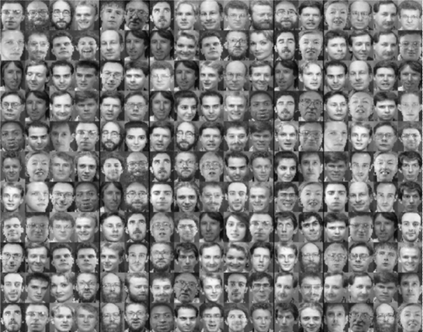
图 ORL人脸数据库
下面是取自人脸的子块,一共取了5000个9×9大小的子块,并进行白化(后面会讲到),这个只是为了使每个像素点的特征独立,但不会像PCA那样降维,后面几节会讲到),子块如下图所示。
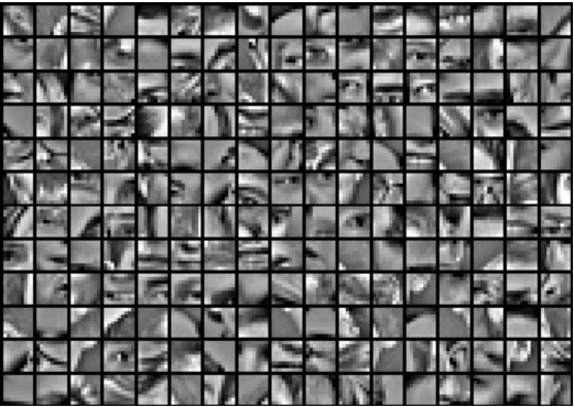
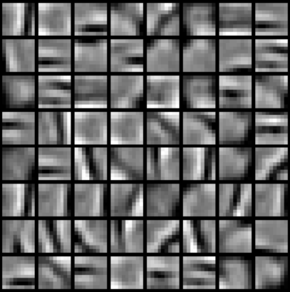
可以看到有人的鼻、眼睛、下巴等子块,下面提供autoencoder(见前面几节)训练滤波器,这是一个自学习网络。训练出64个滤波器如下图所示。
下面分别是任意一张人脸卷积和池化的结果图
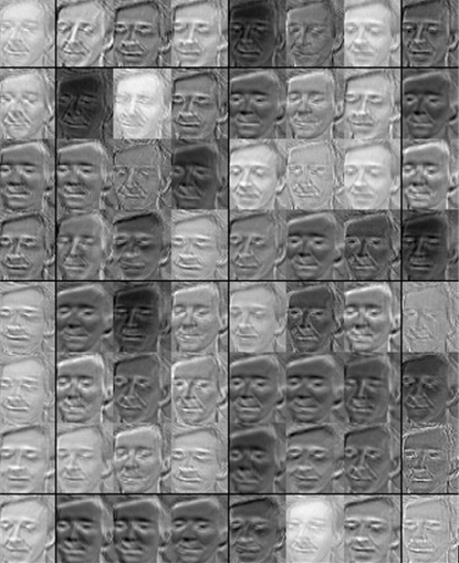
卷积后的结果图
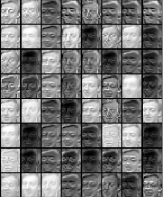
池化后结果图
数据库下载地址:http://www.cl.cam.ac.uk/research/dtg/attarchive/facedatabase.html。 图片大小为112×92,一共200张,可以处理200×10304,并保存为FaceContainer.mat
下面是展示图片结果的函数
display_network.m
<span style="font-family:Times New Roman;font-size:18px;">function [h, array] = display_network(A,sz1,sz, opt_normalize, opt_graycolor, cols, opt_colmajor)
% This function visualizes filters in matrix A. Each column of A is a
% filter. We will reshape each column into a square image and visualizes
% on each cell of the visualization panel.
% All other parameters are optional, usually you do not need to worry
% about it.
% opt_normalize: whether we need to normalize the filter so that all of
% them can have similar contrast. Default value is true.
% opt_graycolor: whether we use gray as the heat map. Default is true.
% cols: how many columns are there in the display. Default value is the
% squareroot of the number of columns in A.
% opt_colmajor: you can switch convention to row major for A. In that
% case, each row of A is a filter. Default value is false.
warning off all
if ~exist('opt_normalize', 'var') || isempty(opt_normalize)
    opt_normalize= true;
end

if ~exist('opt_graycolor', 'var') || isempty(opt_graycolor)
    opt_graycolor= true;
end

if ~exist('opt_colmajor', 'var') || isempty(opt_colmajor)
    opt_colmajor = false;
end
% rescale
A = A - mean(A(:));
if opt_graycolor, colormap(gray); end
% compute rows, cols
[L M]=size(A);
%sz=sqrt(L);
buf=1;
if ~exist('cols', 'var')
    if floor(sqrt(M))^2 ~= M
        n=ceil(sqrt(M));
        while mod(M, n)~=0 && n<1.2*sqrt(M), n=n+1; end
        m=ceil(M/n);
    else
        n=sqrt(M);
        m=n;
    end
else
    n = cols;
    m = ceil(M/n);
end
array=-ones(buf+m*(sz1+buf),buf+n*(sz+buf));
if ~opt_graycolor
    array = 0.1.* array;
end
if ~opt_colmajor
    k=1;
    for i=1:m
        for j=1:n
            if k>M,
                continue;
            end
            clim=max(abs(A(:,k)));
            if opt_normalize
                array(buf+(i-1)*(sz1+buf)+(1:sz1),buf+(j-1)*(sz+buf)+(1:sz))=reshape(A(:,k),sz1,sz)/clim;
            else
                array(buf+(i-1)*(sz1+buf)+(1:sz1),buf+(j-1)*(sz+buf)+(1:sz))=reshape(A(:,k),sz1,sz)/max(abs(A(:)));
            end
            k=k+1;
        end
    end
else
    k=1;
    for j=1:n
        for i=1:m
            if k>M,
                continue;
            end
            clim=max(abs(A(:,k)));
            if opt_normalize
                array(buf+(i-1)*(sz1+buf)+(1:sz1),buf+(j-1)*(sz+buf)+(1:sz))=reshape(A(:,k),sz1,sz)/clim;
            else
                array(buf+(i-1)*(sz1+buf)+(1:sz1),buf+(j-1)*(sz+buf)+(1:sz))=reshape(A(:,k),sz1,sz);
            end
            k=k+1;
        end
    end
end
if opt_graycolor
    h=imagesc(array,'EraseMode','none',[-1 1]);
else
    h=imagesc(array,'EraseMode','none',[-1 1]);
end
axis image off
drawnow;
warning on all</span>
训练滤波器的函数
imageChannels = 1;     % number of channels (rgb, so 3)

patchDim   = 9;          % patch dimension
numPatches = 5000;   % number of patches

visibleSize = patchDim * patchDim * imageChannels;  % number of input units
outputSize  = visibleSize;   % number of output units
hiddenSize  = 64;           % number of hidden units %中间的隐含层还变多了

sparsityParam = 0.035; % desired average activation of the hidden units.
lambda = 3e-3;         % weight decay parameter
beta = 5;              % weight of sparsity penalty term

epsilon = 0.1;           % epsilon for ZCA whitening
load('patchesFace.mat');
meanPatch = mean(patches, 2);  %注意这里减掉的是每一维属性的均值,为什么会和其它的不同呢?
patches = bsxfun(@minus, patches, meanPatch);%每一维都均值化


randsel = randi(size(patches,2),204,1);
% Apply ZCA whitening
sigma = patches * patches' / numPatches;
[u, s, v] = svd(sigma);
ZCAWhite = u * diag(1 ./ sqrt(diag(s) + epsilon)) * u';%求出ZCAWhitening矩阵
patches = ZCAWhite * patches;
figure
display_network(patches(:, randsel),9,9);

%% STEP 1: Learn features
theta = initializeParameters(hiddenSize, visibleSize);

addpath minFunc/
options = struct;
options.Method = 'lbfgs';
options.maxIter = 450;
options.display = 'on';
[optTheta, cost] = minFunc( @(p) sparseAutoencoderLinearCost(p, ...
                                   visibleSize, hiddenSize, ...
                                   lambda, sparsityParam, ...
                                   beta, patches), ...
                              theta, options);%注意它的参数
fprintf('Saving learned features and preprocessing matrices...\n');
save('STL10Features.mat', 'optTheta', 'ZCAWhite', 'meanPatch');
fprintf('Saved\n');

%% STEP 2: Visualize learned features

W = reshape(optTheta(1:visibleSize * hiddenSize), hiddenSize, visibleSize);
b = optTheta(2*hiddenSize*visibleSize+1:2*hiddenSize*visibleSize+hiddenSize);
figure;
display_network( (W*ZCAWhite)',9,9);
save('canshu.mat','W','b');卷积和池化的函数
clear all
clc
load('FaceMat.mat');
load('canshu.mat');
numImages=64;
poolDim=5;
resultDim=21;
resultDim1=17;
face=FaceContainer(15,:);
face=reshape(face,112,92);
face=face/255;


for i=1:64
    w=W(:,i);
    w=reshape(w,8,8);
    resultface=conv2(face,w,'valid');
    bia=repmat(b(i),105,85);
    resultface=bia+resultface;
    featuremap(i,:,:)=resultface;
end
figure('name','featuremap');
featuremap=reshape(featuremap,64,8925);
featuremap=featuremap';
display_network(featuremap(:,1:64),105,85);
featuremap=featuremap';
mat=reshape(featuremap,64,105,85);
for imageNum = 1:numImages
    for poolRow = 1:resultDim
        offsetRow = 1+(poolRow-1)*poolDim;
        for poolCol = 1:resultDim1
            offsetCol = 1+(poolCol-1)*poolDim;
            patch = mat(imageNum,offsetRow:offsetRow+poolDim-1,offsetCol:offsetCol+poolDim-1);
            pooledFeatures(imageNum,poolRow,poolCol) = mean(patch(:));%使用均值pool
        end
    end
end
figure('name','pooledfeaturemap');
pooledFeatures=reshape(pooledFeatures,64,357);
pooledFeatures=pooledFeatures';
display_network(pooledFeatures(:,1:64),21,17);
怀柔风光


 782
782


 被折叠的 条评论
为什么被折叠?
被折叠的 条评论
为什么被折叠?
 到【灌水乐园】发言


