深度学习与Pytorch实战（二）预测房价--线性回归

最新推荐文章于 2025-04-07 09:03:55 发布

volcanical

最新推荐文章于 2025-04-07 09:03:55 发布

阅读量1.8k

点赞数 1

分类专栏： pytorch 文章标签：深度学习 pytorch 线性回归

本文链接：https://blog.csdn.net/huoshanshaohui/article/details/129144678

版权

pytorch 专栏收录该内容

4 篇文章

订阅专栏

PyTorch实例：线性回归

我们将实现一个线性回归模型，并用梯度下降算法求解该模型，从而给出预测曲线。

准备数据

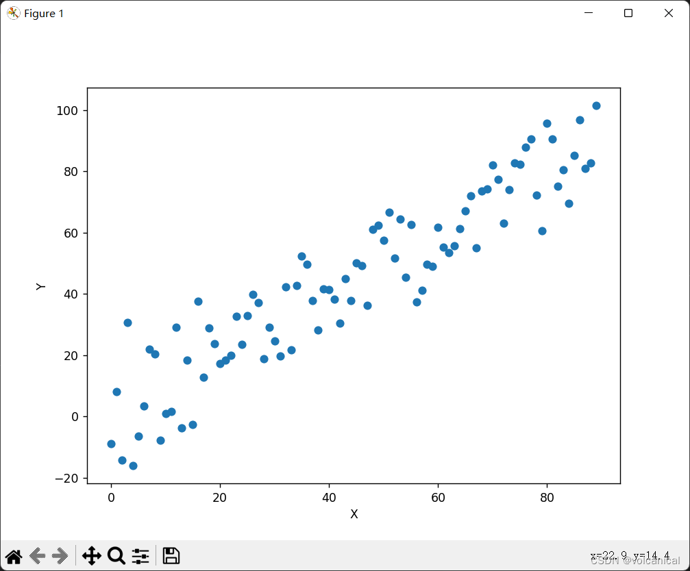
首先我们编造一组数据，假如我们每隔一个月获取一次房价数据，代表0，1，2，3，4……月份，那么我们可以用PyTorch的linespace来构建1~100之间的均匀数字作为时间变量。

import torch
import matplotlib.pyplot as plt
# 0~99月
x = torch.Tensor(range(0, 100))
# 房价
y = x + torch.randn(100)*10

# 测试集与数据集划分
x_train = x[:-10]
x_test = x[-10:]
y_train = y[:-10]
y_test = y[-10:]

plt.figure(figsize=(10, 8))
plt.plot(x_train.numpy(), y_train.numpy(), 'o')
plt.xlabel('X')
plt.ylabel('Y')
plt.show()

* 在这里插入图片描述
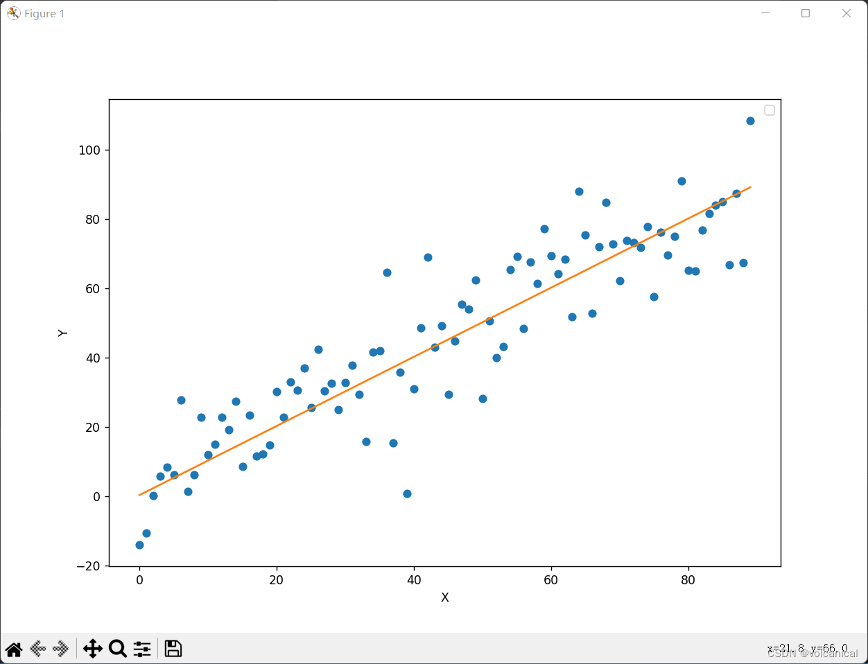
我们希望得到一条尽可能从中间穿越这些数据散点的拟合直线
$y = a x + b$
那么我们需要计算参数a、b的值，我们可以将每一个数据点 $x_i$ 代入这个方程中，计算出一个 $\hat y_i$
我们需要定义一个平均损失函数
$L=\frac{1}{N}\sum^{N}_{i}(y_i-\hat y_i)^2 = \frac{1}{N}\sum^{N}_{i}(y_i-ax_i-b)^2$
并让这个损失函数尽可能小，其中N是所有点的个数100。
我们利用梯度下降法反复迭代a和b，从而让L越来越小。在计算的过程中，我们需要计算出L对a,b的偏导数，利用Pytorch的backward可以非常方便地计算出这两个偏导数。于是我们只需要一步一步地更新a和b就可以了。

训练

首先我们需要定义两个自动微分变量a和b，然后通过求解Loss对a和b的梯度来更新参数a和b。

注意：a和b是自动微分变量，不能直接对自动微分变量进行数值更新，只能对他的data属性进行更新。


a = torch.rand(1, requires_grad=True)
b = torch.rand(1, requires_grad=True)

learning_rate = 0.0001

for i in range(1000):
    predictions = a * x_train + b
    loss = torch.mean((predictions - y_train) ** 2)
    print('loss:', loss)
    loss.backward()

    a.data.add_(-learning_rate*a.grad.data)
    b.data.add_(-learning_rate*b.grad.data)

    a.grad.data.zero_()
    b.grad.data.zero_()

x_data = x_train.numpy()
plt.figure(figsize=(10,7))
xplot = plt.plot(x_data, y_train.data.numpy(), 'o')
yplot = plt.plot(x_data, a.data.numpy()*x_data+b.data.numpy())
plt.xlabel('X')
plt.ylabel('Y')
str1 = str(a.data.numpy())[0] + 'x' + str(b.data.numpy())[0]

plt.legend([xplot, yplot],['Data', str1])
plt.show()

在这里插入图片描述

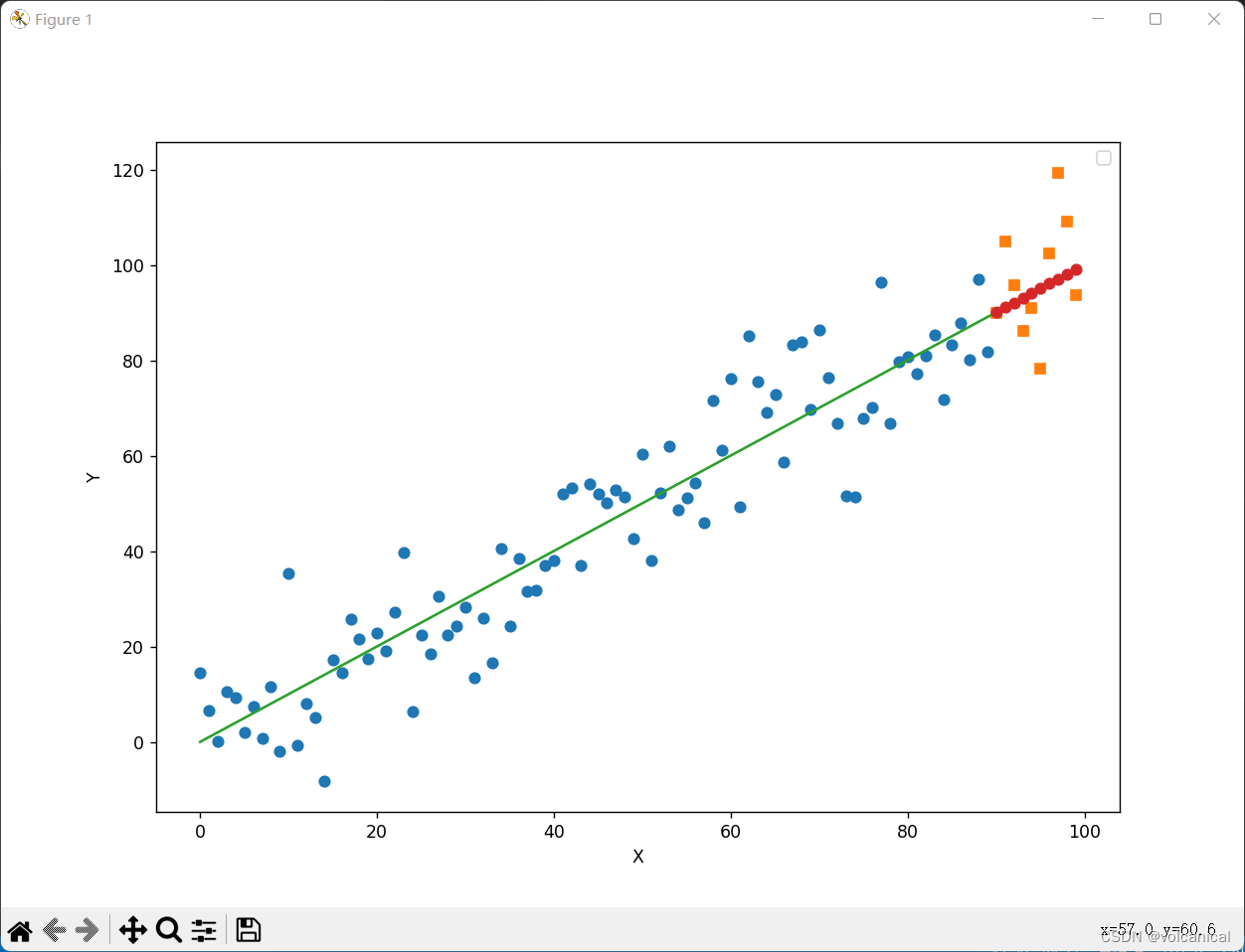
预测

最后一步，我们在保留的10个测试集上进行测试

x_data = x_train.data.numpy()
x_pred = x_test.data.numpy()
plt.figure(figsize=(10,7))
plt.plot(x_data, y_train.numpy(), 'o')
plt.plot(x_pred, y_test.numpy(), 's')
x_data = np.r_[x_data, x_test.numpy()]
plt.plot(x_data, a.data.numpy()*x_data+b.data.numpy())
plt.plot(x_pred, a.data.numpy()*x_pred+b.data.numpy(), 'o')

plt.xlabel('X')
plt.ylabel('Y')
str1 = str(a.data.numpy())[0] + 'x' + str(b.data.numpy())[0]
plt.legend([xplot, yplot],['Data', str1])
plt.show()