均值、方差、标准差、均方根、均方误差、均方根误差的区别与联系

均值、方差、标准差、均方根、均方误差、均方根误差的区别与联系

The mean, variance, and standard deviation are the most basic statistical measures. The mean均值${\mu }_x$, and variance方差 ${\sigma }_x^2$, of a set of $n$ observations, $x_i$, are defined as
$${\mu }_x=\frac{1}{n}\sum _{i=1}^n{x}_i,{\sigma }_x^2=\frac{1}{n}\sum _{i=1}^n{\left(x_i-{\mu }_x\right)}^2=\frac{1}{n}\sum _{i=1}^n{x}_i^2-{\mu }_x^2.$$
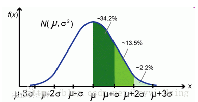
They may also be written as $\mu (x)$​ and ${\sigma }^2(x)$​, respectively The standard deviation (SD) 标准差 ${\sigma }_x$​ or $\sigma (x)$​​, is simply the square root of the variance, 既然有了方差来描述变量与均值的偏离程度，那又搞出来个标准差干什么呢？原因是：方差与我们要处理的数据的量纲是不一致的，虽然能很好的描述数据与均值的偏离程度，但是处理结果是不符合我们的直观思维的。举个例子：一个班级里有60个学生，平均成绩是70分，标准差是9，方差是81，成绩服从正态分布，那么我们通过方差不能直观的确定班级学生与均值到底偏离了多少分，通过标准差我们就很直观的得到学生成绩分布在[61,79]范围的概率为0.6826，即约等于下图中的34.2%*2

while the root mean square (RMS) is
$$r_x=\sqrt{\frac{1}{n}\sum _{i=1}^n{x}_i^2}.$$
The mean and variance form part of a wider set of statistical measures called moments. The $k^{\text{th }}$-order moment （k阶矩） $m_k$, and central moment**（k阶中心矩） $c_k$**, are defined as
$$m_k(x)=\frac{1}{n}\sum _{i=1}^n{x}_i^k,c_k(x)=\frac{1}{n}\sum _{i=1}^n{\left(x_i-{\mu }_x\right)}^k.$$
Note that $c_1$ is always zero. The mean is the first-order moment and the variance the second-order central moment. The RMS is the square root of the second-order moment. The third-order central moment is known as the skew.请注意，$c_1$始终为零，均值是一阶矩，方差是二阶中心矩，均方根是二阶矩的平方根，三阶中心力矩称为偏斜。

Suppose the observations, $x_i$, are taken from a population with distribution $X$. Unbiased estimates of the mean, ${\mu }_X$, and variance, ${\sigma }_X^2$, of the population’s distribution are
$${\hat{\mu }}_X={\mu }_x,{\hat{\sigma }}_X^2=\frac{n}{n-1}{\sigma }_x^2.$$
**一组向量观测值的平均值就是各分量平均值的向量，向量分布的方差的等价物是协方差矩阵。**The mean of a set of vector observations is simply the vector of the means of the components. The equivalent of the variance for a vector distribution is the covariance matrix, $\mathbf{C}$ (P may also be used). If $\mathbf{x}$ is an $m$-component vector, ${\mathbf{C}}_{\mathbf{x}}$ is an $m\times m$ matrix. A covariance matrix is symmetric with the diagonal elements corresponding to the variances of the components of the vector it describes and the off-diagonal elements giving the covariance of each pair of components.Where the components of the vector are uncorrelated, the off diagonal elements （非对角元素）of $\mathbf{C}$ will tend to zero as the number of observations increases.（协方差矩阵是对称的，对角线元素对应于它所描述的矢量的分量的方差，非对角线元素给出每对分量的协方差。在向量分量不相关的情况下，随着观测次数的增加，$\mathbf{C}$的非对角线元素将趋于零） The mean, ${\mathbf{\mu }}_{\mathbf{x}}$, and covariance, ${\mathbf{C}}_{\mathbf{x}}$, of a set of $n$ observations, ${\mathbf{x}}_i$, are
$${\mathbf{\mu }}_{\mathbf{x}}=\frac{1}{n}\sum _{i=1}^n{\mathbf{x}}_i,{\mathbf{C}}_{\mathbf{x}}=\frac{1}{n}\sum _{i=1}^n\left({\mathbf{x}}_i-{\mathbf{\mu }}_{\mathbf{x}}\right){\left({\mathbf{x}}_i-{\mathbf{\mu }}_{\mathbf{x}}\right)}^{\mathrm{T}}=\frac{1}{n}\sum _{i=1}^n{\mathbf{x}}_i{\mathbf{x}}_i^{\mathrm{T}}-{\mathbf{\mu }}_{\mathbf{x}}{\mathbf{\mu }}_{\mathbf{x}}^{\mathrm{T}}.$$
Higher-order moments can also describe vector data, noting that a $k^{\text{th }}$-order moment or central moment of a vector is a $k^{\text{th }}$-order tensor.高阶矩也可以描述向量数据，注意向量的$k$阶矩或中心矩是$k$阶张量。

均方误差、均方根误差

**均方根误差RMSE：**各个数据偏离真实值的距离的平方和，再开方

**均方误差MSE：**各个数据偏离真实值的距离的平方和

**标准差：**各个数据偏离均值的距离的平方，再开方（也叫均方差）

**方差：**各个数据偏离均值的距离的平方
$$\begin{array}{c}MSE=\frac{\sum {\left(x_i-{\hat{x}}_i\right)}^2}{N}\\ RMSE=\sqrt{\frac{1}{N}\sum {\left(x_i-{\hat{x}}_i\right)}^2}\end{array}$$

均方根值（RMS）：也称有效值
$$X_{RMS}=\sqrt{\frac{1}{N}\left(X_1^2+X_2^2+\dots X_N^2\right)}$$
比如幅度为100V而占空比为0.5的方波信号，如果按平均值计算，它的电压只有50V，而按均方根值计算则有70.71V。这是为什么呢？举一个例子，有一组100伏的电池组，每次供电10分钟之后停10分钟，也就是说占空比为一半。如果这组电池带动的是10Ω电阻，供电的10分钟产生10A的电流和1000W的功率，停电时电流和功率为零。

也就是说均方根值反映的是有效值而不是平均值，它具有一定的实际（物理）意义。**均方误差（Mean Squared Error）、均方根误差（Root Mean Square Error）**在公式形式上与方差、标准差并没有太大区别，但是从物理意义上有明显差异。区别在于前者应用情景存在一个真实值，其衡量的是各数据偏离真实值的情况，