This series of articles are the study notes of " Machine Learning ", by Prof. Andrew Ng., Stanford University. This article is the notes of week 3, Solving the Problem of Overfitting Part II. This article contains some topic about how to implementation linear regression with regularization to addressing overfitting.
Regularized Linear Regression
1. Cost Function of Linear Regression with Regularization
For linear regression, we have previously worked out two learning algorithms. One based on gradient descent and one based on the normal equation. In this video, we'll take those two algorithms and generalize them to the case of regularized linear regression.
Original cost function of linear regressionwithout regularization:

Cost function of linear regression with regularization:
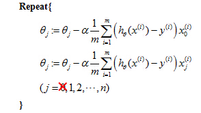
Let's take a look at the gradient descent algorithm below. Previously, we were using gradient descent for the original cost function without the regularization term. And we had the following algorithm, for regular linear regression, without regularization, we would repeatedly update the parameters theta J as follows for J =0, 1, 2, ... n.
Gradient descent for linear regression (without regularization term):

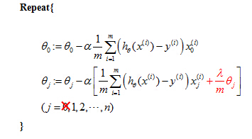
Let me take this and just write the case for theta 0 separately. So I'm just going to write the update for theta 0 separately than for the update for the parameters 1, 2, 3, and so on up to n. And so this is, I haven't changed anything yet. This is just writing the update for theta 0 separately from the updates for theta 1, theta 2, theta 3, up to theta n.

Gradient descent for linear regression (with regularization term):

Analysis of the update effect for θ after adding the regularization term
And if you calculate the partial derivative,you will find out that the term in the square bracket is the partial derivative of the regularization form of cost function J(θ).

And, the first term is the partial derivative
2. Normal equation
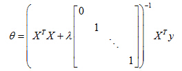
And in order to minimize the cost function J, we found that one way to do so is to set theta to be equal to this. And what this value for theta does is this minimizes the cost function J of theta, when we were not using regularization.
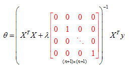
Now if you are using regularization, then this formula changes as follows. Inside this parenthesis, you end up with a matrix like this. 0, 1, 1, 1, and so on, 1, until the bottom. So this thing over here is a matrix whose upper left-most entry is 0. There are ones on the diagonals, and then zeros everywhere else in this matrix.
E.g. n=2

But as a example, if n = 2, then this matrix is going to be a three by three matrix. More generally, this matrix is an(n+1) by (n+1) dimensional matrix.
but it is possible to prove that if you are using the new definition of J of theta, with the regularization objective, then this new formula for theta is the one that we give you, the global minimum ofJ(θ).
3. Non-invertibility
So finally I want to just quickly describe the issue of non-invertibility.
If you have fewer examples than features, than this matrix, X transpose X will be non-invertible, or singular. Or the other term for this is the matrix will be degenerate. And if you implement this in Octave anyway and you use the pinv function to take the pseudo inverse,it will kind of do the right thing, but it's not clear that it would give you a very good hypothesis, even though numerically the Octave pinv function will give you a result that kinda makes sense.
Suppose m≤n, (m is the number of examples, n is the number of features)

if (XTX)is non-invertible or singular.
Fortunately, regularization also takes care of this for us. And concretely, so long as the regularization parameter λ is strictly greater than 0, it is actually possible to prove that this matrix,X transpose X plus lambda times this funny matrix here, it is possible to prove that this matrix will not be singular and that this matrix will be invertible:
If λ > 0,

The matrix in the above equation will not be non-invertible or singular.


 201
201

 被折叠的 条评论
为什么被折叠?


