


4.2 多项式回归
以多元线性回归和特征工程的思想得到一种称为多项式回归的新算法。可以拟合非线性曲线。
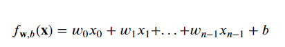
这是线性回归时使用的预测模型:
先看看按照以前的线性回归方法的效果:
# create target data
x = np.arange(0, 20, 1)
y = 1 + x**2
X = x.reshape(-1, 1)

model_w,model_b = run_gradient_descent_feng(X,y,iterations=1000, alpha = 1e-2)

plt.scatter(x, y, marker='x', c='r', label="Actual Value"); plt.title("no feature engineering")
plt.plot(x,X@model_w + model_b, label="Predicted Value");  plt.xlabel("X"); plt.ylabel("y"); plt.legend(); plt.show()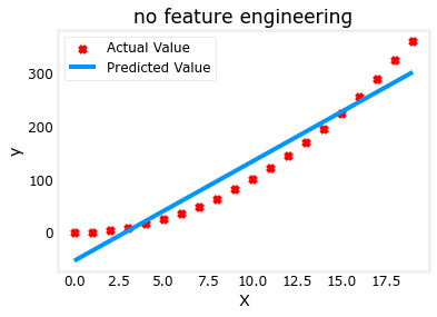
以前的效果
我们需要多项式特征,因此我们进行上面提到的特征工程,调整x的次数:
# create target data
x = np.arange(0, 20, 1)
print(f"X: {x}")
y = 1 + x**2

# Engineer features
X = x**2      #<-- added engineered feature
X = X.reshape(-1, 1) #X should be a 2-D Matrix X应为二维矩阵
print(f"X: {X}")
model_w,model_b = run_gradient_descent_feng(X, y, iterations=100000, alpha = 1e-5)
plt.scatter(x, y, marker='x', c='r', label="Actual Value"); plt.title("Added x**2 feature")
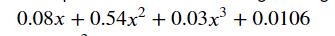
plt.plot(x, np.dot(X,model_w) + model_b, label="Predicted Value"); plt.xlabel("x"); plt.ylabel("y"); plt.legend(); plt.show()拟合出来的式子为:
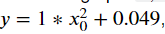
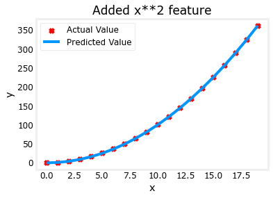
特征工程后
4.3 特征选择
Above, we knew that an 𝑥2x2 term was required. It may not always be obvious which features are required. One could add a variety of potential features to try and find the most useful. For example, what if we had instead tried : 𝑦=𝑤0𝑥0+𝑤1𝑥21+𝑤2𝑥32+𝑏y=w0x0+w1x12+w2x23+b ?
上面,我们知道𝑥需要2个学期。需要哪些功能可能并不总是显而易见的。人们可以添加各种潜在功能来尝试并找到最有用的功能。例如,如果我们尝试:𝑦=𝑤0𝑥0+𝑤1.𝑥21+𝑤2.𝑥32+𝑏 ?
# create target data
x = np.arange(0, 20, 1)
y = x**2

# engineer features .
X = np.c_[x, x**2, x**3]   #<-- added engineered feature
#print(f"X: {X}")
model_w,model_b = run_gradient_descent_feng(X, y, iterations=100000, alpha=1e-7)
plt.scatter(x, y, marker='x', c='r', label="Actual Value"); plt.title("x, x**2, x**3 features")
plt.plot(x, X@model_w + model_b, label="Predicted Value"); plt.xlabel("x"); plt.ylabel("y"); plt.legend(); plt.show()
Iteration 0, Cost: 1.14029e+03
Iteration 10000, Cost: 7.90568e+01
Iteration 20000, Cost: 1.62482e+01
Iteration 30000, Cost: 3.34903e+00
Iteration 40000, Cost: 6.99857e-01
Iteration 50000, Cost: 1.55758e-01
Iteration 60000, Cost: 4.39818e-02
Iteration 70000, Cost: 2.09930e-02
Iteration 80000, Cost: 1.62388e-02
Iteration 90000, Cost: 1.52295e-02
w,b found by gradient descent: w: [1.49e-01 9.76e-01 8.68e-04], b: 0.0187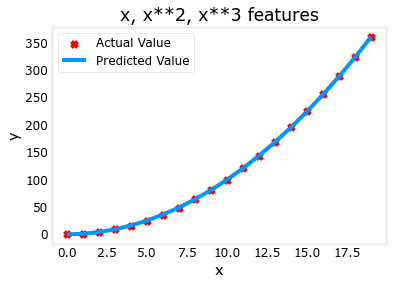
拟合出的式子为:
梯度下降通过强调其相关参数为我们选择“正确”的特征。
4.4 多项式特征和线性回归特征之间的联系
以上,多项式特征是根据它们与目标数据的匹配程度来选择的。考虑这一点的另一种方式是注意,一旦我们创建了新特征,我们仍然在使用线性回归。考虑到这一点,最佳特征将是相对于目标的线性特征。这一点最好通过一个例子来理解。
# create target data
x = np.arange(0, 20, 1)
y = x**2

# engineer features .
X = np.c_[x, x**2, x**3]   #<-- added engineered feature
X_features = ['x','x^2','x^3']
#fig, ax = plt.subplots(1,3),其中参数1和3分别代表子图的行数和列数,一共有 1x3 个子图像。函数返回一个figure图像和子图ax的array列表。
fig,ax=plt.subplots(1, 3, figsize=(12, 3), sharey=True)
for i in range(len(ax)):
ax[i].scatter(X[:,i],y)
ax[i].set_xlabel(X_features[i])
ax[0].set_ylabel("y")
plt.show()
Above, it is clear that the 𝑥 2x2 feature mapped against the target value 𝑦 y is linear. Linear regression can then easily generate a model using that feature.
上面,很明显𝑥根据目标值映射2个特征𝑦 是线性的。然后,线性回归可以使用该特性轻松生成模型。
4.5 复杂函数拟合
通过特征工程,甚至可以对非常复杂的功能进行建模:
x = np.arange(0,20,1)
y = np.cos(x/2)

X = np.c_[x, x**2, x**3,x**4, x**5, x**6, x**7, x**8, x**9, x**10, x**11, x**12, x**13]
X = zscore_normalize_features(X)

model_w,model_b = run_gradient_descent_feng(X, y, iterations=1000000, alpha = 1e-1)

plt.scatter(x, y, marker='x', c='r', label="Actual Value"); plt.title("Normalized x x**2, x**3 feature")
plt.plot(x,X@model_w + model_b, label="Predicted Value"); plt.xlabel("x"); plt.ylabel("y"); plt.legend(); plt.show()

Iteration         0, Cost: 2.24887e-01
Iteration    100000, Cost: 2.31061e-02
Iteration    200000, Cost: 1.83619e-02
Iteration    300000, Cost: 1.47950e-02
Iteration    400000, Cost: 1.21114e-02
Iteration    500000, Cost: 1.00914e-02
Iteration    600000, Cost: 8.57025e-03
Iteration    700000, Cost: 7.42385e-03
Iteration    800000, Cost: 6.55908e-03
Iteration    900000, Cost: 5.90594e-03
w,b found by gradient descent: w: [-1.61e+00 -1.01e+01  3.00e+01 -6.92e-01 -2.37e+01 -1.51e+01  2.09e+01
 -2.29e-03 -4.69e-03  5.51e-02  1.07e-01 -2.53e-02  6.49e-02], b: -0.0073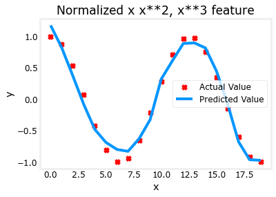
五、使用Scikit Learn的线性回归
有一个开源的、商用的机器学习工具包,叫做scikit-learn。此工具包包含您将在本课程中使用的许多算法的实现。
关于StandardScaler()函数:sklearn中StandardScaler()
关于SGDRegressor:随机梯度线性回归,随机梯度下降是不将所有样本都进行计算后再更新参数,而是选取一个样本,计算后就更新参数。
关于LinearRegression:也是线性回归模型,这里没用,可以自己查。
import numpy as np
from my_Function.lab_utils_multi import load_house_data
np.set_printoptions(precision=2)
from sklearn.linear_model import LinearRegression, SGDRegressor
#Standardization标准化:将特征数据的分布调整成标准正太分布,也叫高斯分布,也就是使得数据的均值维0,方差为1.
from sklearn.preprocessing import StandardScaler
import matplotlib.pyplot as plt
dlblue = '#0096ff'; dlorange = '#FF9300'; dldarkred='#C00000'; dlmagenta='#FF40FF'; dlpurple='#7030A0';
plt.style.use('./deeplearning.mplstyle')
梯度下降 Scikit learn有一个梯度下降回归模型sklearn.liner_model.SGDRegressor。与您以前的梯度下降实现一样,该模型在标准化输入时表现最好。sklearn.preprrocessing.StandardScaler将像以前的实验室一样执行z评分标准化。这里称为“标准评分”。以下代码参考博主:https://blog.csdn.net/qq_52466006 在此谢谢大佬~🙏
if __name__ == '__main__':
# data = np.loadtxt('houses.txt', dtype=np.float32, delimiter=',')
X_train = np.array([[2104, 5, 1, 45], [1416, 3, 2, 40], [852, 2, 1, 35]])
Y_train = np.array([460, 232, 178])
#X_train = data[:, :4]
X_train, y_train = load_house_data()
X_features = ['size(sqft)', 'bedrooms', 'floors', 'age']
X_features = ['size(sqft)', 'bedrooms', 'floors', 'age']
#y_train = np.ravel(data[:, 4:5]) # 把Y转为一维数组
# 使用sklearn进行Z-score标准化
scaler = StandardScaler()
X_norm = scaler.fit_transform(X_train) # 标准化训练集X
# print(X_norm)
# 创建回归拟合模型
sgdr = SGDRegressor(max_iter=1000) # 设置最大迭代次数
sgdr.fit(X_norm, y_train)
print(sgdr)
print(f"完成的迭代次数: {sgdr.n_iter_}, 权重更新数: {sgdr.t_}")
# 查看参数
b_norm = sgdr.intercept_
w_norm = sgdr.coef_
print(f"SGDRegressor拟合参数: w: {w_norm}, b:{b_norm}")
print(f"之前自己编写的线性回归拟合参数: w: [110.61 -21.47 -32.66 -37.78], b: 362.23")
# 使用sgdr.predict()进行预测
y_pred_sgd = sgdr.predict(X_norm)
# 使用w和b进行预测
y_pred = np.dot(X_norm, w_norm) + b_norm
print(f"使用 np.dot() 预测值是否与sgdr.predict预测值相同: {(y_pred == y_pred_sgd).all()}")
print(f"训练集预测:\n{y_pred[:4]}")
print(f"训练集真实值\n{y_train[:4]}")
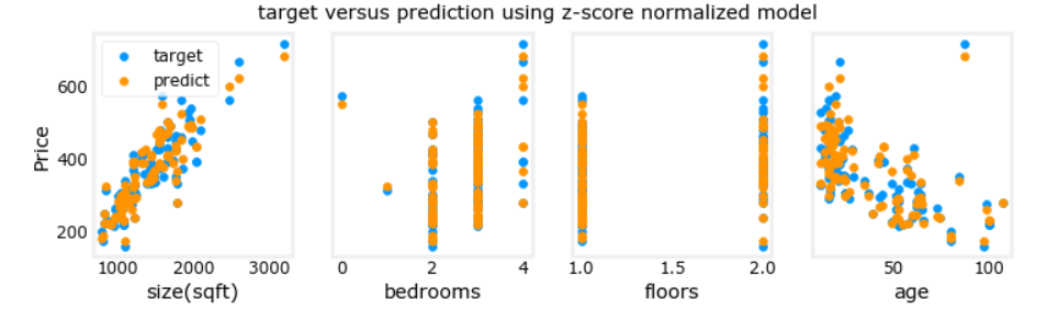
# 绘制训练集与预测值匹配情况
fig, ax = plt.subplots(1, 4, figsize=(12, 3), sharey=True)
for i in range(len(ax)):
ax[i].scatter(X_train[:, i], y_train, label='target')
ax[i].set_xlabel(X_features[i])
ax[i].scatter(X_train[:, i], y_pred, color='orange', label='predict')
ax[0].set_ylabel("Price")
ax[0].legend()
fig.suptitle("target versus prediction using z-score normalized model")
plt.show()运行结果:
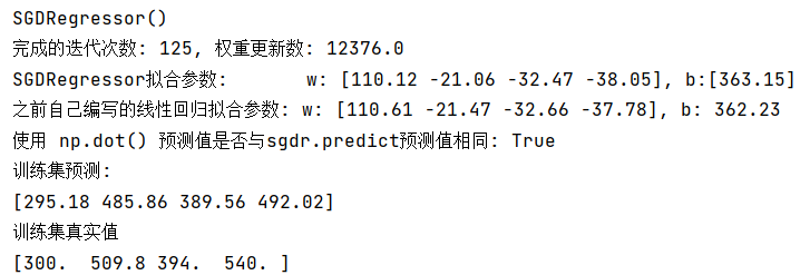
训练集预测值与实际值对比:


 212
212

 被折叠的 条评论
为什么被折叠?
被折叠的 条评论
为什么被折叠?
 到【灌水乐园】发言


