week2作业

C1_W2_test.py

import matplotlib.pyplot as plt
from test_Function.utils import  *
from test_Function.C1_W2_testFunction import  *
import copy
import math
#%matplotlib inline

if __name__ == '__main__':
    x_train, y_train = load_data()
    # print x_train
    print('-----------------查看数据（x_train是一个城市的人口，ytrain是那个城市一家餐馆的利润。利润为负值表示亏损。）-----------------')
    print("x_train的类型:",type(x_train))
    print("x_train的前五个元素是:\n", x_train[:5])
    # print y_train
    print("y_train的类型:",type(y_train))
    print("y_train的前五个元素是:\n", y_train[:5])

    print('-----------------检查变量的维度-----------------')
    '''检查变量的维度

       熟悉数据的另一个有用方法是查看其维度。

       请打印x_train和y_train的形状，并查看数据集中有多少训练示例。
    '''
    print('The shape of x_train is:', x_train.shape)
    print('The shape of y_train is: ', y_train.shape)
    print('训练数据的数量（m）:', len(x_train))

    '''可视化数据

      通过可视化来理解数据通常很有用。

      对于这个数据集，您可以使用散点图来可视化数据，因为它只有两个属性要绘制（利润和人口）。

      你在现实生活中遇到的许多其他问题都有两个以上的属性（例如，人口、家庭平均收入、月利润、月销售额）。当你有两个属性以上时，你仍然可以使用散点图来查看每对属性之间的关系。'''
    # 创建数据的散点图。要将标记更改为红色“x”，
    # 我们使用了“标记”和“c”参数
    plt.scatter(x_train, y_train, marker='x', c='r')

    # Set the title
    plt.title("Profits vs. Population per city")
    # Set the y-axis label
    plt.ylabel('Profit in $10,000')
    # Set the x-axis label
    plt.xlabel('Population of City in 10,000s')
    plt.show()

    print('-----------------计算代价总和-----------------')
    '''我们的目标是建立一个线性回归模型来拟合这些数据。
      线性回归的模型函数是一个从“x”（城市人口）映射到“y”（您餐厅在该城市的月利润）的函数，表示为𝑓𝑤,𝑏(𝑥)=𝑤𝑥+𝑏
      𝑐𝑜𝑠𝑡(𝑖)=(𝑓𝑤𝑏−𝑦(𝑖))2
      返回所有示例的总成本 𝐽(𝐰,𝑏)=12𝑚∑𝑖=0𝑚−1𝑐𝑜𝑠𝑡(𝑖)
      使用该模型，您可以输入一个新城市的人口，并让该模型估计您的餐厅在该城市的潜在月度利润。
      '''

# Compute cost with some initial values for paramaters w, b
initial_w = 2
initial_b = 1

cost = compute_cost(x_train, y_train, initial_w, initial_b)
print(type(cost))
print(f'Cost at initial w (zeros): {cost:.3f}')

print('-----------------计算梯度-----------------')

# Compute and display gradient with w initialized to zeroes
initial_w = 0.2
initial_b = 0.2

tmp_dj_dw, tmp_dj_db = compute_gradient(x_train, y_train, initial_w, initial_b)
print('Gradient at initial w, b (zeros):', tmp_dj_dw, tmp_dj_db)

print('-----------------使用批次梯度下降找到合适的w,b-----------------')
# initialize fitting parameters. Recall that the shape of w is (n,)
initial_w = 0.
initial_b = 0.

# some gradient descent settings
iterations = 1500
alpha = 0.01

w,b,_,_ = gradient_descent(x_train ,y_train, initial_w, initial_b,
                     compute_cost, compute_gradient, alpha, iterations)
print("w,b found by gradient descent:", w, b)


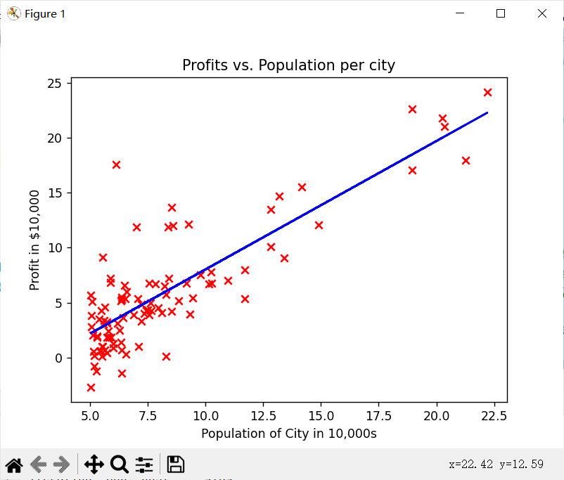
'''现在我们将使用梯度下降的最终参数来绘制线性拟合。 回想一下，我们可以得到单个示例的预测𝑓(𝑥(𝑖))=𝑤𝑥(𝑖)+𝑏 .
 为了计算整个数据集的预测，我们可以循环所有训练示例，并计算每个示例的预测。这显示在下面的代码块中。'''
m = x_train.shape[0]
predicted = np.zeros(m)

for i in range(m):
    predicted[i] = w * x_train[i] + b

print('-----------------绘制预测值以查看线性拟合。-----------------')
# Plot the linear fit
plt.plot(x_train, predicted, c = "b")

# Create a scatter plot of the data.
plt.scatter(x_train, y_train, marker='x', c='r')

# Set the title
plt.title("Profits vs. Population per city")
# Set the y-axis label
plt.ylabel('Profit in $10,000')
# Set the x-axis label
plt.xlabel('Population of City in 10,000s')
plt.show()

'''我们的最终价值𝑤,𝑏 也可以用来预测利润。让我们来预测35000人和70000人的地区的利润。 该模型以10000人的城市人口为输入。 
因此，35000人可以转化为np.array模型的输入（[3.5]） 类似地，70000人可以被转换为np.array（[7.]）模型的输入'''
print('-----------------预测利润情况-----------------')
predict1 = 3.5 * w + b
print('人口数为 35,000, 预测利润为 $%.2f' % (predict1*10000))

predict2 = 7.0 * w + b
print('人口数为 70,000, 预测利润为 $%.2f' % (predict2*10000))

C1_W2_testFunction.py

import copy
import math

def compute_cost(x, y, w, b):
    """
    Computes the cost function for linear regression.

    Args:
        x (ndarray): Shape (m,) Input to the model (Population of cities)
        y (ndarray): Shape (m,) Label (Actual profits for the cities)
        w, b (scalar): Parameters of the model

    Returns
        total_cost (float):使用w，b作为线性回归参数的成本以拟合x和y中的数据点
    """
    # number of training examples
    m = x.shape[0]

    # You need to return this variable correctly
    total_cost = 0

    ### START CODE HERE ###
    for i in range(m):
        f_wb_i = x[i] * w + b
        total_cost = total_cost + (f_wb_i - y[i]) ** 2
    total_cost = total_cost / (2 * m)
    ### END CODE HERE ###

    return total_cost


# GRADED FUNCTION: compute_gradient
def compute_gradient(x, y, w, b):
    """
    Computes the gradient for linear regression
    Args:
      x (ndarray): Shape (m,) Input to the model (Population of cities)
      y (ndarray): Shape (m,) Label (Actual profits for the cities)
      w, b (scalar): Parameters of the model
    Returns
      dj_dw (scalar): The gradient of the cost w.r.t. the parameters w
      dj_db (scalar): The gradient of the cost w.r.t. the parameter b
     """

    # Number of training examples
    m = x.shape[0]

    # You need to return the following variables correctly
    dj_dw = 0
    dj_db = 0

    ### START CODE HERE ###
    for i in range(m):
        f_wb_i = w * x[i] + b
        dj_db = dj_db + (f_wb_i - y[i])
        dj_dw = dj_dw + (f_wb_i - y[i]) * x[i]
    dj_dw = dj_dw / m
    dj_db = dj_db / m

    ### END CODE HERE ###

    return dj_dw, dj_db


def gradient_descent(x, y, w_in, b_in, cost_function, gradient_function, alpha, num_iters):
    """
    Performs batch gradient descent to learn theta. Updates theta by taking
    num_iters gradient steps with learning rate alpha

    Args:
      x :    (ndarray): Shape (m,)
      y :    (ndarray): Shape (m,)
      w_in, b_in : (scalar) Initial values of parameters of the model
      cost_function: function to compute cost
      gradient_function: function to compute the gradient
      alpha : (float) Learning rate
      num_iters : (int) number of iterations to run gradient descent
    Returns
      w : (ndarray): Shape (1,) Updated values of parameters of the model after
          running gradient descent
      b : (scalar)                Updated value of parameter of the model after
          running gradient descent
    """

    # number of training examples
    m = len(x)

    # An array to store cost J and w's at each iteration — primarily for graphing later
    J_history = []
    w_history = []
    w = copy.deepcopy(w_in)  # avoid modifying global w within function
    b = b_in

    for i in range(num_iters):

        # Calculate the gradient and update the parameters
        dj_dw, dj_db = gradient_function(x, y, w, b)

        # Update Parameters using w, b, alpha and gradient
        w = w - alpha * dj_dw
        b = b - alpha * dj_db

        # Save cost J at each iteration
        if i < 100000:  # prevent resource exhaustion
            cost = cost_function(x, y, w, b)
            J_history.append(cost)

        # Print cost every at intervals 10 times or as many iterations if < 10
        if i % math.ceil(num_iters / 10) == 0:
            w_history.append(w)
            print(f"Iteration {i:4}: Cost {float(J_history[-1]):8.2f}   ")

    return w, b, J_history, w_history  # return w and J,w history for graphing

运行结果：