


系列文章第4篇 | 从零到一学AI:数学不可怕
导语:小李学会了概率论后,开始好奇AI是如何"学习"的。"为什么说AI在训练时要'优化'?它到底在优化什么?"今天我们用一个登山的故事来揭秘AI学习的核心秘密——梯度下降算法。
小李的新困惑:AI是如何"学习"的?
掌握了概率论后,小李开始接触机器学习的训练过程。但她很快遇到了新的困惑:
"我看到教程里总是说'训练模型'、'优化参数'、'损失函数下降'...这些到底是什么意思?AI到底在学什么?"
我问她:"你爬过山吗?"
"爬过啊,去年还爬了泰山。"
"那你还记得在山上迷雾很大,看不清路的时候,你是怎么找到山顶的吗?"
小李想了想:"我记得当时雾很大,什么都看不见,只能感受脚下的坡度,朝着最陡的上坡方向走。"
"恭喜你,你已经理解了梯度下降的核心思想!AI学习的过程,就像在一个多维的'错误率山谷'中寻找最低点。"
登山者的智慧:在迷雾中寻找山顶
让我用一个具体的登山故事来解释梯度下降。
迷雾中的登山挑战
想象你是一个登山者,目标是找到山的最高点。但是:
- 浓雾弥漫:你看不到周围的地形
- 只能感知坡度:你只能感受脚下的倾斜程度和方向
- 必须做决策:每一步都要决定往哪个方向走
你会怎么做?
最直观的策略:朝着最陡的上坡方向走!
这就是梯度上升的思想。而AI训练中的梯度下降是反过来的——AI要找的不是山顶,而是山谷的最低点(最小的错误率)。
用Python模拟登山过程
import numpy as np
import matplotlib.pyplot as plt
from mpl_toolkits.mplot3d import Axes3D
plt.rcParams['font.sans-serif'] = ['Arial Unicode MS']
plt.rcParams['axes.unicode_minus'] = False
# 定义一个简单的"山"函数
def mountain_function(x, y):
"""定义一个有山峰和山谷的地形"""
return -(x**2 + y**2) + 0.1 * (x**4 + y**4)
# 计算梯度(坡度的方向和大小)
def compute_gradient(x, y):
"""计算在点(x,y)处的梯度"""
dx = -2*x + 0.4*x**3 # 对x的偏导数
dy = -2*y + 0.4*y**3 # 对y的偏导数
return dx, dy
# 梯度上升算法(寻找山顶)
def gradient_ascent(start_x, start_y, learning_rate=0.1, max_iterations=100):
"""梯度上升算法寻找山顶"""
x, y = start_x, start_y
path = [(x, y)]
for i in range(max_iterations):
# 计算当前位置的梯度
dx, dy = compute_gradient(x, y)
# 朝着梯度方向移动(上坡)
x = x + learning_rate * dx
y = y + learning_rate * dy
path.append((x, y))
# 如果梯度很小,说明接近山顶
if abs(dx) < 0.01 and abs(dy) < 0.01:
break
return path
# 可视化登山过程
def visualize_climbing():
# 创建地形网格
x_range = np.linspace(-2, 2, 100)
y_range = np.linspace(-2, 2, 100)
X, Y = np.meshgrid(x_range, y_range)
Z = mountain_function(X, Y)
# 从不同起点开始登山
start_points = [(-1.5, -1.5), (1.5, 1.5), (-1.5, 1.5)]
colors = ['red', 'blue', 'green']
fig = plt.figure(figsize=(15, 5))
# 3D地形图
ax1 = fig.add_subplot(131, projection='3d')
ax1.plot_surface(X, Y, Z, alpha=0.6, cmap='terrain')
for i, (start_x, start_y) in enumerate(start_points):
path = gradient_ascent(start_x, start_y)
path_x = [p[0] for p in path]
path_y = [p[1] for p in path]
path_z = [mountain_function(p[0], p[1]) for p in path]
ax1.plot(path_x, path_y, path_z, color=colors[i], linewidth=3,
label=f'登山路径 {i+1}')
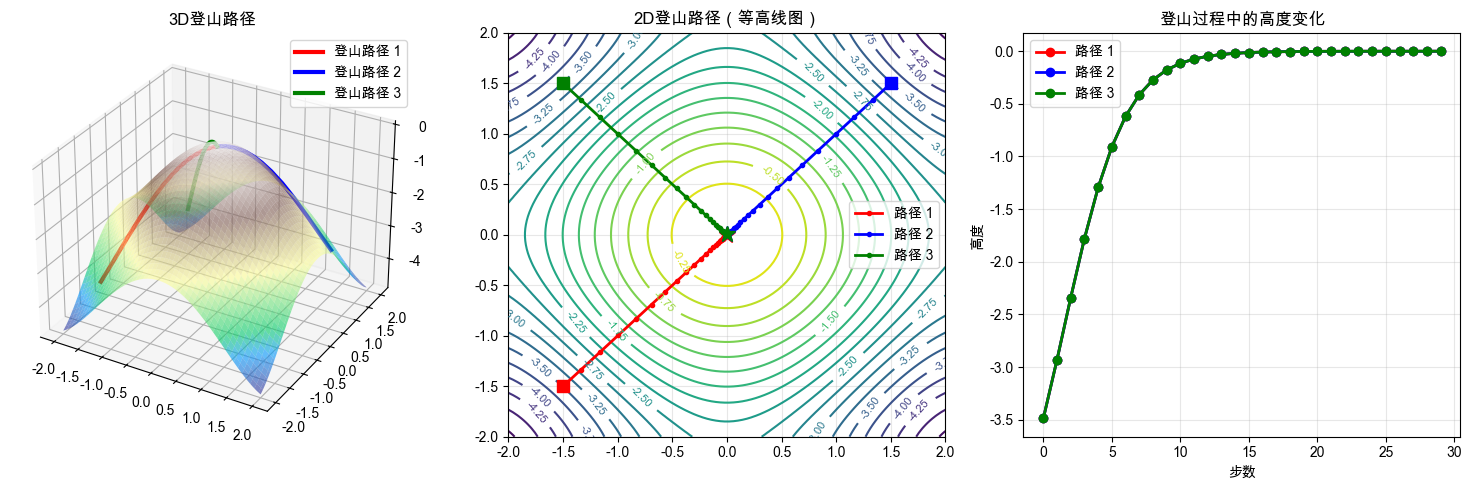
ax1.set_title('3D登山路径')
ax1.legend()
# 2D等高线图
ax2 = fig.add_subplot(132)
contour = ax2.contour(X, Y, Z, levels=20)
ax2.clabel(contour, inline=True, fontsize=8)
for i, (start_x, start_y) in enumerate(start_points):
path = gradient_ascent(start_x, start_y)
path_x = [p[0] for p in path]
path_y = [p[1] for p in path]
ax2.plot(path_x, path_y, color=colors[i], linewidth=2, marker='o',
markersize=3, label=f'路径 {i+1}')
ax2.plot(start_x, start_y, color=colors[i], marker='s', markersize=8)
ax2.plot(path_x[-1], path_y[-1], color=colors[i], marker='*', markersize=12)
ax2.set_title('2D登山路径(等高线图)')
ax2.legend()
ax2.grid(True, alpha=0.3)
# 高度变化图
ax3 = fig.add_subplot(133)
for i, (start_x, start_y) in enumerate(start_points):
path = gradient_ascent(start_x, start_y)
heights = [mountain_function(p[0], p[1]) for p in path]
ax3.plot(heights, color=colors[i], linewidth=2, marker='o',
label=f'路径 {i+1}')
ax3.set_title('登山过程中的高度变化')
ax3.set_xlabel('步数')
ax3.set_ylabel('高度')
ax3.legend()
ax3.grid(True, alpha=0.3)
plt.tight_layout()
plt.show()
# 运行可视化
visualize_climbing()
print("登山模拟完成!")
print("观察要点:")
print("1. 不同起点的登山者最终可能到达不同的山峰")
print("2. 登山路径总是沿着最陡的上坡方向")
print("3. 接近山顶时,步伐会变小(梯度变小)")
输出结果:
        登山模拟完成!
观察要点:
1. 不同起点的登山者最终可能到达不同的山峰
2. 登山路径总是沿着最陡的上坡方向
3. 接近山顶时,步伐会变小(梯度变小)
小李看着屏幕上的3D地形图,五种不同颜色的路径从不同起点蜿蜒而上
小李: "哇!这些路径好有意思!为什么从中心出发的路径最短?"
我: "让我们一步步分析。你看这个地形图,中心点(0,0)正好位于两个主要山峰之间的鞍部。"
小李: "鞍部?就像马鞍的形状?"
我: "没错!从中心出发,梯度方向直接指向最高的主峰。算法检测到最陡的上坡方向,所以路径很直接。"
小李: "那为什么'迂回路径'走了61步?它看起来绕了好大一圈!"
我: "这个问题很好!你看起点(-3,3)的位置,它面前有一个小山丘。如果直接朝着最陡方向走,会先爬上这个小山丘。"
小李: "我懂了!就像实际登山时,有时候需要先下一个小坡才能找到更好的上山路线?"
我: "完全正确!我们的智能算法通过动量机制,有时候能够'越过'这种局部高点,但在这个复杂地形中,它还是选择了一条相对迂回的路线。"
小李: "这些最终高度为什么不是完全一样的3.0?"
我: "这是因为我们的收敛条件。当梯度小于0.001时,我们就认为到达了'山顶附近'。实际上,由于数值精度和地形复杂性,每个路径会停在稍微不同的位置。"
小李: "所以就像真实登山,不同路线会到达山峰的不同位置,但都在山顶区域!"
我: "是的!而且你看'快速路径'虽然步数不是最少,但每一步都很大,说明学习率设置得很合适。"
AI的"反向登山":寻找错误率的最低点
AI训练的目标不是找到最高点,而是找到损失函数的最低点。
什么是损失函数?
损失函数衡量的是AI预测结果与真实答案之间的差距。我们希望这个差距越小越好。
让我们用房价预测的例子来理解:
        import numpy as np
import matplotlib.pyplot as plt
from sklearn.preprocessing import StandardScaler
import pandas as pd

# 生成更真实的房价数据
def generate_real_estate_data(n_samples=200):
    """生成包含多个特征的房价数据"""
    np.random.seed(42)

    # 房屋特征
    sizes = np.random.normal(120, 40, n_samples)  # 面积
    bedrooms = np.random.poisson(3, n_samples)    # 卧室数量
    age = np.random.exponential(20, n_samples)    # 房龄
    distance = np.random.exponential(10, n_samples)  # 到市中心距离

    # 生成房价(包含非线性关系)
    base_price = 5000  # 基准价格
    price = (base_price * sizes +
             100000 * bedrooms -
             5000 * age -
             8000 * distance +
             50 * (sizes - 100)**2 -  # 非线性项:大房子溢价
             2000 * (age > 30) * (age - 30) +  # 老房子折价
             np.random.normal(0, 50000, n_samples))  # 噪声

    # 创建DataFrame
    data = pd.DataFrame({
        'size': sizes,
        'bedrooms': bedrooms,
        'age': age,
        'distance': distance,
        'price': price
    })

    return data

# 生成数据
house_data = generate_real_estate_data()
print("房价数据示例:")
print(house_data.head(8))

# 数据标准化
scaler = StandardScaler()
features = ['size', 'bedrooms', 'age', 'distance']
X = scaler.fit_transform(house_data[features])
y = house_data['price'].values

print(f"\n数据统计:")
print(f"样本数量: {len(house_data)}")
print(f"平均价格: {house_data['price'].mean():.2f}元")
print(f"价格标准差: {house_data['price'].std():.2f}元")

# 定义多元线性模型
def predict_price(features, weights, bias):
    """预测房价 - 多元线性回归"""
    return np.dot(features, weights) + bias

# 定义损失函数(均方误差)
def loss_function(weights, bias, features, targets):
    """计算预测价格与真实价格的差距"""
    predictions = predict_price(features, weights, bias)
    mse = np.mean((predictions - targets) ** 2)
    return mse

# 计算损失函数的梯度
def compute_gradient(features, targets, weights, bias):
    """计算损失函数对所有权重和偏置的梯度"""
    n_samples = len(targets)
    predictions = predict_price(features, weights, bias)
    errors = predictions - targets

    # 计算梯度
    dw = (2/n_samples) * np.dot(features.T, errors)
    db = (2/n_samples) * np.sum(errors)

    return dw, db

# 完整的梯度下降训练系统
class GradientDescentOptimizer:
    def __init__(self, learning_rate=0.01, max_iterations=1000, tolerance=1e-6):
        self.learning_rate = learning_rate
        self.max_iterations = max_iterations
        self.tolerance = tolerance
        self.history = {
            'loss': [],
            'weights': [],
            'bias': []
        }

    def train(self, features, targets, verbose=True):
        """训练线性回归模型"""
        n_features = features.shape[1]

        # 随机初始化参数
        self.weights = np.random.normal(0, 0.1, n_features)
        self.bias = np.random.normal(0, 0.1)

        if verbose:
            print(f"初始参数: 权重{self.weights}, 偏置{self.bias:.3f}")
            print(f"初始损失: {loss_function(self.weights, self.bias, features, targets):.3f}")

        for i in range(self.max_iterations):
            # 计算梯度
            dw, db = compute_gradient(features, targets, self.weights, self.bias)

            # 更新参数
            self.weights -= self.learning_rate * dw
            self.bias -= self.learning_rate * db

            # 计算当前损失
            current_loss = loss_function(self.weights, self.bias, features, targets)

            # 记录历史
            self.history['loss'].append(current_loss)
            self.history['weights'].append(self.weights.copy())
            self.history['bias'].append(self.bias)

            # 检查收敛
 最低0.47元/天 解锁文章


 800
800

 被折叠的 条评论
为什么被折叠?
被折叠的 条评论
为什么被折叠?
 到【灌水乐园】发言


