使用python写神经网络模型之分类器

最新推荐文章于 2024-08-05 23:33:38 发布

Tiger-Li

最新推荐文章于 2024-08-05 23:33:38 发布

阅读量1.2k

点赞数 1

分类专栏：机器学习

机器学习专栏收录该内容

112 篇文章 25 订阅

订阅专栏

http://blog.csdn.net/eric_doug/article/details/51769644

使用python写神经网络模型之分类器

标签： python 神经网络

2016-06-27 17:13 783人阅读评论(0) 收藏举报

 
  分类： 
 
  机器学习

 版权声明：本文为博主原创文章，原文链接地址: http://blog.csdn.net/eric_doug

 目录(?)[+]

最近在尝试将所有的机器学习与深度学习的模型用Python来实现，大致的学习思路如下：

分类器
回归与预测
时间序列

所有的模型先用 Python语言实现，然后用Tensorflow的实现。

1 数据集

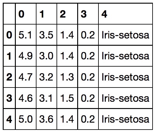
本文开始以UCI中的Iris数据集作为训练数据集和测试时间集。该数据集给出了花萼(sepal)的长度和宽度以及花瓣(petal)的长度和宽度，根据这4个特征训练模型，预测花的类别(Iris Setosa，Iris Versicolour，Iris Virginica)。

# 包引入
import pandas as pd
import numpy as np
import matplotlib.pyplot as plt
import os
df = pd.read_csv('https://archive.ics.uci.edu/ml/machine-learning-databases/iris/iris.data', header=None)
df.head(10)
   
   1
2
3
4
5
6
7
   
   1
2
3
4
5
6
7

iris

1.1 数据处理

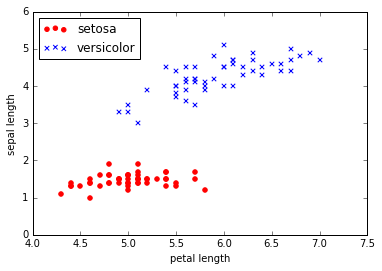
我们提取前100个样本(50个Iris Setosa和50个Iris Versicolour)，并将不同的样本类别标注为1(Iris Versicolour)和-1(Iris Setosa)；然后，将花萼的长度和花瓣的长度作为特征。大致处理如下：

y = df.iloc[0:100, 4].values  # 预测标签向量
y = np.where(y == 'Iris-setosa', -1, 1)
X = df.iloc[0:100, [0,2]].values  # 输入特征向量

# 使用散点图可视化样本
plt.scatter(X[:50, 0], X[:50,1], color='red', marker='o', label='setosa')
plt.scatter(X[50:100, 0], X[50:100, 1], color='blue', marker='x', label='versicolor')
plt.xlabel('petal length')
plt.ylabel('sepal length')
plt.legend(loc='upper left')
plt.show
   
   1
2
3
4
5
6
7
8
9
10
11
   
   1
2
3
4
5
6
7
8
9
10
11

sample_scatter

2 模型

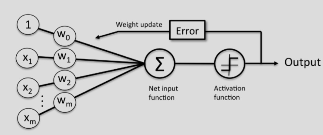
2.1 神经网络模型

2.1.1 模型实现

我们可以将该问题转化为一个二分类的任务，因此，可以将1与-1作为类别标签。从而激活函数可以表示如下:

ϕ (z) = {1 - 1, z \geq 0, z < 0

大致的模型结构如下：
nn1

class Perceptron(object):
    """
    Parameters
    ------------
    eta : float
        学习率 (between 0.0 and 1.0)
    n_iter : int
        迭代次数
    Attributes
    -----------
    w_ : 1d-array
        权重
    errors_ : list
        误差
    """
    def __init__(self, eta=0.01, n_iter=10):
        self.eta = eta
        self.n_iter = n_iter

    def fit(self, X, y):
        self.w_ = np.zeros(1 + X.shape[1])
        self.errors_ = []

        for _ in range(self.n_iter):
            errors = 0
            for xi, target in zip(X, y):
                update = self.eta * (target - self.predict(xi))
                self.w_[1:] += update * xi
                self.w_[0] += update
                errors += int(update != 0.0)
            self.errors_.append(errors)
        return self

    def net_input(self, X):
        return np.dot(X, self.w_[1:]) + self.w_[0]

    def predict(self, X):
        return np.where(self.net_input(X) >= 0.0, 1, -1)
   
   1
2
3
4
5
6
7
8
9
10
11
12
13
14
15
16
17
18
19
20
21
22
23
24
25
26
27
28
29
30
31
32
33
34
35
36
37
38
   
   1
2
3
4
5
6
7
8
9
10
11
12
13
14
15
16
17
18
19
20
21
22
23
24
25
26
27
28
29
30
31
32
33
34
35
36
37
38

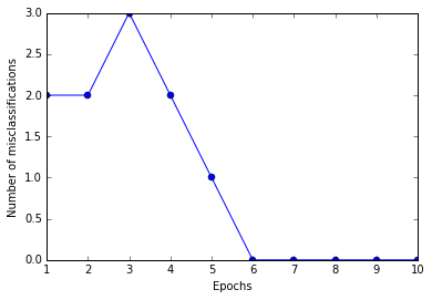
2.1.2 模型训练

ppn = Perceptron(eta=0.1, n_iter=10)
ppn.fit(X, y)
   
   1
2
   
   1
2

2.1.3 模型验证

误差分析

plt.plot(range(1, len(ppn.errors_) + 1), ppn.errors_, marker='o')
plt.xlabel('Epochs')
plt.ylabel('Number of misclassifications')
plt.show()
   
   1
2
3
4
   
   1
2
3
4

nn1_errors

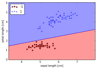
可视化分类器

from matplotlib.colors import ListedColormap
def plot_decision_regions(X, y, classifier, resolution=0.01):
    """
    可视化分类器
    :param X:  样本特征向量
    :param y:  样本标签向量
    :param classifier: 分类器
    :param resolution: 残差
    :return:
    """

    markers = ('s', 'x', 'o', '^', 'v')
    colors = ('red', 'blue', 'lightgreen', 'gray', 'cyan')
    cmap = ListedColormap(colors[:len(np.unique(y))])

    x1_min, x1_max = X[:, 0].min() - 1, X[:, 0].max() + 1
    x2_min, x2_max = X[:, 1].min() - 1, X[:, 1].max() + 1
    xx1, xx2 = np.meshgrid(np.arange(x1_min, x1_max, resolution), np.arange(x2_min, x2_max, resolution))

    Z = classifier.predict(np.array([xx1.ravel(), xx2.ravel()]).T)
    Z = Z.reshape(xx2.min(), xx2.max())

    plt.contourf(xx1, xx2, Z, alpha=0.4, cmap=cmap)
    plt.xlim(xx1.min(), xx1.max())
    plt.ylim(xx2.min(), xx2.max())

    for idx, cl in enumerate(np.unique(y)):
        plt.scatter(x=X[y == cl, 0], y=X[y == cl, 1], alpha=0.8, c=cmap(idx), marker=markers[idx], label=cl)

# 调用可视化分类器函数
plot_decision_regions(X, y, classifier=ppn)
plt.xlabel('sepal length [cm]')
plt.ylabel('petal length [cm]')
plt.legend(loc='upper left')
plt.show()
   
   1
2
3
4
5
6
7
8
9
10
11
12
13
14
15
16
17
18
19
20
21
22
23
24
25
26
27
28
29
30
31
32
33
34
35
   
   1
2
3
4
5
6
7
8
9
10
11
12
13
14
15
16
17
18
19
20
21
22
23
24
25
26
27
28
29
30
31
32
33
34
35