李沐动手学深度学习08线性回归+基础优化算法

08线性回归+基础优化算法

线性模型中n维输入就可以用向量表示，n维权重也可以用向量表示，以及一个标量偏差（这其实就是普通的变量，例如y=ax+b中的b）。通过向量表示就可以是y=<w,x>+b（内积+b）。

衡量预测质量：损失函数=1/2(真实值-估计值)^2，前面的常量是为了求导的时候可以凑1。这样的函数成为平方损失

训练损失中，1/2是平方损失中原本就有的，1/n是为了求每个训练样本的平均损失；<xi,w>是求每个样本的估计值，右侧的向量版本可能更容易理解。

最小化损失就是为了求解局部最优的w和b

• 线性回归是有显示解的。
• 线性模型可以看作单层神经网络。

梯度下降

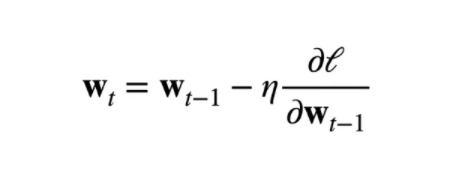
可以简单思考一下这里为什么是-号，因为我们要求的是整个损失函数的最小值，右侧是学习率(这是一个超参数，需要人为设定)和偏导。学习率太大会震荡无法到达局部最优，太小效率会很低。

一般来说每次计算梯度都不会对全部样本进行计算，这个过程非常慢，所以一般进行小批量的样本计算，就是随机采样b个版本来近似损失，b就是批量大小，这是另一个超参数。批量太小无法充分利用资源，太大会导致内存资源消耗增加。

线性回归从零实现

import matplotlib as matplotlib
import random
import torch
from d2l import torch as d2l


# 随机生成数据
def synthetic_data(w, b, num_examples):
    """生成 y=wx + b + 噪声"""
    x = torch.normal(0, 1, (num_examples, len(w)))  # 返回一个张量，正态分布N(0,1)
    y = torch.matmul(x, w) + b  # 向量的乘积，再加一个偏差b
    y += torch.normal(0, 0.01, y.shape) # 添加一个随机噪音，均值为0，方差为0.01，形状为y.shape
    return x, y.reshape((-1, 1))    # reshape-1表示自动匹配


# 生成batch_size大小的小批量
def data_iter(batch_size, features, labels):
    num_examples = len(features)
    indices = list(range(num_examples))
    # 这些样本是随机读取的，没有特定的顺序
    random.shuffle(indices) # 随机打乱下标，这样就可以继续随机读取了
    for i in range(0, num_examples, batch_size):
        batch_indices = torch.tensor(
            indices[i:min(i+batch_size, num_examples)]
        )
        # 这里的batch_indices是选取的下标
        yield features[batch_indices], labels[batch_indices]    # yield和return差不多，但是这个返回的是一个生成器


# 线性回归模型
def linreg(x, w, b):
    return torch.matmul(x, w) + b


# 损失函数
def squared_loss(y_hat, y):
    return (y_hat - y.reshape(y_hat.shape)) ** 2 / 2


# 优化算法 小批量随机梯度下降
def sgd(params, lr, batch_size):
    with torch.no_grad():   # 更新的时候不要进行梯度计算
        for param in params:
            param -= lr * param.grad / batch_size   # 这里依据导数对权重参数进行更新操作
            param.grad.zero_()


if __name__ == '__main__':
    true_w = torch.tensor([2, -3.4])
    true_b = 4.2
    features, labels = synthetic_data(true_w, true_b, 1000)

    print("features:", features, "\nlabel:", labels)
    d2l.set_figsize()
    d2l.plt.scatter(features[:, (1)].detach().numpy(),
                    labels.detach().numpy(), 1)
    d2l.plt.show()  # 数据的临时展示

    batch_size = 10
    for x,y in data_iter(batch_size, features, labels):
        print(x,"\n", y)
        break

    w = torch.normal(0, 0.01, size=(2, 1), requires_grad=True)
    b = torch.zeros(1, requires_grad=True)

    # 模型训练
    lr = 0.03   # 学习率大小
    num_epochs = 3  # 整个训练集遍历3次
    net = linreg    # 这个是训练的网络
    loss = squared_loss #损失函数的计算方法

    for epoch in range(num_epochs):
        for x,y in data_iter(batch_size, features, labels):
            l = loss(net(x, w, b), y)

            l.sum().backward()  # 求和以后算梯度
            sgd([w, b], lr, batch_size)

        with torch.no_grad():   # 不需要计算梯度
            train_l = loss(net(features, w, b), labels)
            print(f'epoch {epoch+1}, loss{float(train_l.mean()):f}')

    print(f'w的估计误差：{true_w - w.reshape(true_w.shape)}')
    print(f'b的估计误差：{true_w - b}')

简化线性回归

import numpy as np
import torch
from torch.utils import data
from d2l import torch as d2l
from torch import nn


# 构造一个pytorch的数据迭代器
def load_array(data_arrays, batch_size, is_train=True):
    dataset = data.TensorDataset(*data_arrays)
    # 每次随机从dataset中挑选batch_size个样本，shuffle=is_train就是是否需要随机打乱
    return data.DataLoader(dataset, batch_size, shuffle=is_train)


if __name__ == '__main__':
    true_w = torch.tensor([2, -3.4])
    true_b = 4.2
    features, labels = d2l.synthetic_data(true_w, true_b, 1000)

    batch_size = 10
    data_iter = load_array((features, labels), batch_size)

    next(iter(data_iter))

    net = nn.Sequential(nn.Linear(2, 1)) # 参数表示输入输出维度,net中本身就带有模型参数

    # weight就是访问w,data就是访问w的值，normal就是使用正态分部用来替换掉data中的值
    net[0].weight.data.normal_(0, 0.01)
    net[0].bias.data.fill_(0)

    # 计算均方误差，平方误差
    loss = nn.MSELoss()

    trainer = torch.optim.SGD(net.parameters(), lr=0.03)

    num_epochs = 3
    for epoch in range(num_epochs):
        for x,y in data_iter:
            l = loss(net(x), y)
            trainer.zero_grad()
            l.backward()
            trainer.step()  # 有梯度以后对参数进行更新
        l = loss(net(features), labels) # 计算在整个训练情况下的平均loss
        print(f'epoch {epoch+1}, loss{l:f}')